In this article, I shall be discussing the existing underground cable fault location methods. Faults in a cable may vary widely, and similar faults may show different symptoms depending upon the cable type, operating voltage, soil condition, and so on. Faults can be considered to be shorts, opens, or nonlinear.
A short is defined as a fault when the conductor is shorted to the ground, neutral, or another phase with a low impedance path. This type of fault is also referred to as a shunt fault.
An open fault is defined as when the conductor is physically broken and no current flows at or beyond the point of the break.
The nonlinear type of fault exhibits the characteristics of an unfaulted conductor at low voltages but shows a short at operating or higher voltages. This nonlinear fault is also known as a high-resistance fault.
Underground Cable Fault Location Methods
Underground cable fault location methods can be divided into two general categories:
- terminal techniques and
- tracing techniques.
Terminal Techniques
These involve measuring some electrical characteristics of the faulted conductor from one of the cable terminals and comparing it with unfaulted conductor characteristics in terms of the distance of the fault.
The effectiveness of this method is a function of the accuracy of installation records. These methods do not pinpoint faults, however, they localize faults.
The terminal techniques category can be further subdivided in terms of the actual methods employed, which are
- bridge,
- radar, and
- resonance methods.
Bridge Method of Cable Fault Location
Various types of bridge configurations may be used to locate faults in underground cables. The most common is the Murry loop and the capacitance bridge.
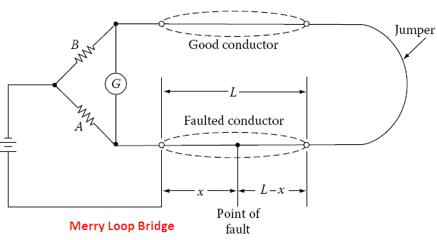
The Murry loop bridge uses a proportional measure so that it is not necessary to know the actual cable resistance. Its principle of operation involves a continuous loop of cable to form the two arms of the bridge. It is necessary to have an unfaulted conductor available to form such a loop. When the bridge is balanced, the distance to the fault can be found by the following expression:
X = 2L [A ÷ (A+ B)]
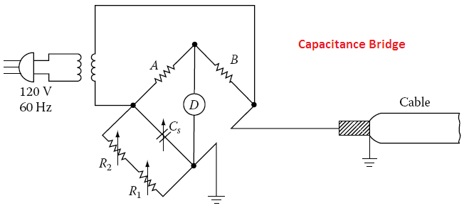
The capacitance bridge technique simply measures the capacitance from one end of the faulted cable to the ground and compares it in terms of the distance with the capacitance of the unfaulted conductor in the same cable.
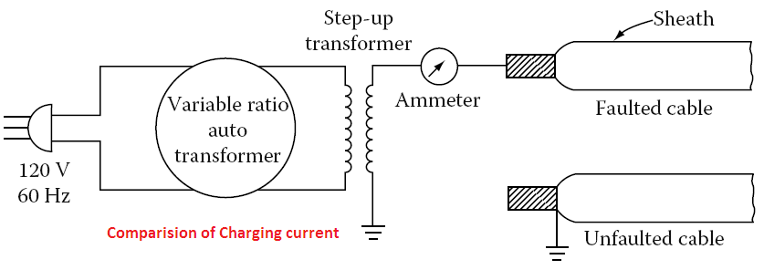
In place of a bridge, the charging current of faulted cable and unfaulted cable can be compared, using several hundred volts or several thousand volts of 60 Hz or 50 Hz supply voltage. The distance L1 to the fault can be found by the following expression:
L1 = L2(I1÷I2)
Where I1 is the current in the faulted conductor, I2 is the current in the unfaulted conductor, and L2 is the length of the unfaulted conductor.
The application of bridge methods can be used on all types of cables. The Murry loop bridge is effective where the parallel fault resistance is low or the bridge voltage is high. It is ineffective on open faults. Open faults can be located with the capacitance bridge.
Radar Method
The radar (reflection or pulse-echo) method is based upon the measurement of the time that it takes the pulse to reach a fault and reflect. The distance d of the fault for uniform cable can be obtained from the expression d = vt/2, where v is propagation velocity and t is the time it takes for the pulse to travel to the fault and back.
There are two types of output pulse duration employed in radar methods. The short-duration pulse type is most commonly used in radar test sets for testing power cables. The pulse duration is short in comparison to propagation time to the fault.
The width of the pulse is usually wide enough to be able to be observed on the oscilloscope. Practically, the pulse width must be greater than 1% of the transit time for the entire cable length under test. Most commercial equipment has provisions for changing the pulse width depending on cable length. The pulse magnitudes are very small, usually on the order of a few volts.
The short pulse does not lend itself well to the interpretation of data because of reflections from splices or the non-uniformity of cable size. The long-pulse system employs long step pulses as compared to the transit time of the signal from one end of the cable to the fault and back. Any discontinuities in the cable are seen as changes in the voltage level of the step pulse. It is easier to interpret the data in a long-pulse system; that is, the faults can be differentiated from splices, and changes in cable size can be easily observed.
In radar systems, the scope trace shows the transmitted and reflected signal. The separation of the two signals is measured and multiplied by the scope calibration to give the transit time. The reflected wave can be expressed in terms of the transmitted wave and circuit constants as follows:
lr = [(R – Z) ÷ (R + Z)]lt
Where lr is the reflected wave, lt is the transmitted wave R is the resistance at the end of the line Z is the impedance of the line.
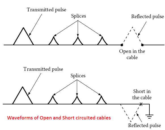
If the line is open-circuited, then R = ∝ and the reflected wave is lr = lt . Therefore, the reflected wave is of the same magnitude and same polarity as the transmitted wave.
If the line is short-circuited, R = 0 and the reflected wave is lr = −lt . Therefore, the reflected wave, in this case, is of equal magnitude to the transmitted wave but 180° out of phase. These two conditions are shown in Figure given below.
The radar can be applied to all types of cable systems provided the propagation velocity is constant along the length of the cable. The radar system does not work very well with nonlinear faults. However, it can be used when the nonlinear fault impedance is burned to a low resistance value. To provide this flexibility, three major variations of radar systems are available:
- the arc radar system,
- the free oscillation system, and
- the differential radar system.
The arc radar system uses an HV pulse system so that the high-impedance (nonlinear) faults can be burned down until they appear as shorts and the radar pulse can be reflected from the arc short.
The free oscillation system is used for high-impedance faults in which the breakdown of the arc causes a pulse to be transmitted down the cable. In this method, the cable end at which measurements are made is terminated in a high impedance (i.e., open) so that the pulse formed at the arc is reflected from the open end to the short at the arc and back to the open end.
This reflection back and forth continues until the energy is completely absorbed by the cable. The period of the signal is four times the transit time of the pulse as it travels the distance of the fault. Therefore, the distance to the fault is one-fourth the product of the propagation velocity and transit time.
The differential radar system is applicable for fault location on branched systems. It is based on the fact that a faulted cable phase is almost always paralleled by an identical unfaulted phase.
The radar prints of the two phases will be identical, except that part of the print is associated with the fault itself. The differential radar signal is applied to both phases simultaneously and the return signals are subtracted. The radar pulse input shows at the point of the fault.
Resonance Method
The resonance technique is based on the principle of wave reflection. The resonance method for fault location measures the frequency at which the length of the cable between the terminal and the fault resonates. The resonant frequency is inversely proportional to the wavelength. The distance d of the fault can be determined by the following expression:
d = V ÷ frN
Where, V is the propagation velocity, fr is the resonant frequency and N is the number of quarter- or half-wavelengths.
Normally, quarter-wave resonance is used for locating shorts, in which case N = 4, and half-wave resonance is used for locating opens, in which case N = 2.
The resonance technique uses a frequency generator (or oscillator), which is connected to the end of the faulted cable. The frequency is varied until resonance is reached. At resonance, the voltage changes rapidly from the voltage at non-resonance frequency. The voltage will increase for shorts and decrease for opens, respectively.
The minimum frequency required is determined by the cable length, and the maximum frequency is determined by the distance to the nearest point at which a fault may occur.
For an insulated cable, the phase shift governs the speed of the transmitted and reflected wave to the fault and back. The phase shift is a function of the dielectric constant of the insulating material.
Usually, the velocity of propagation for insulated cables varies between one-third and one-fourth of the velocity of propagation of bare conductors, which is 984 ft./μs. Therefore, the velocity for cable will be somewhere between 328 and 246 ft./μs. Therefore, for each insulating medium, its dielectric constant must be known for fault location.
The relationship between frequency and distance to the fault is given by the following expression:
This method can be used on all types of cables and works well on branched systems. It does not work very well with nonlinear faults.
d = 466N ÷ frK
Where, N is the number of quarter- or half-wavelengths, fr is the resonance frequency (MHz), K is the dielectric constant of cable and d is the distance to the fault.
Tracer Techniques
Trace techniques are those that involve placing an electrical signal on the faulted feeder from one or both ends, which can be traced along the cable length and detected at the fault by a change in signal characteristics. The following methods are available under this classification:
- Tracing current
- Audio frequency (tone tracing)
- Impulse (thumper) voltage
- Earth gradient
Tracing current method
In this application, both DC and AC methods are employed. This method can be used for fault location on a branched system as well as on a straight uniform cable system.
The fault current is injected into the circuit formed by the faulted conductor and the ground, and a detector is then used to measure the cable current at selected manhole locations.
This technique is applicable where fault resistance is low or the voltage of the test set is high enough to send sufficient current through the faulted conductor. This method is mostly applicable for duct line installations because it is sufficient to know the fault between manholes since the entire section of cable between manholes must be replaced when faulted.
The major consideration for use of this method is to assure that a substantial amount of return current is via the ground path rather than the neutral. If all the current flows through the neutral, the current seen by the detector is canceled for three-conductor cables, and there is no output from the detector.
This is very important for insulated neutral cables, such as PILC, where it is necessary to assure neutral to ground contact between the point of the measurement and the fault.
The tracing DC method uses a modulated DC power supply ranging from 500 V to 20 kV and current ranging from 0.25 to 12.5 A. The detector can be either an electromagnetically coupled circuit using a pickup coil and a galvanometer to detect directional signal, or test prods may be used on the cable sheath, using a drop-of-potential circuit with a galvanometer for signal-direction detection.
The tracing AC method uses a 25 or 60 Hz modulated transmitter consisting of 100% induction regulation or a constant-current transformer. The detectors can consist of either a split-core current transformer and an ammeter or a sheath drop detection circuit consisting of test prods and a milli-voltmeter. The test set range is from 15 to 450 kVA, and audio amplifiers are available with output meters, headsets, or speakers. This method applies to direct buried, insulated cables for a short-to-ground fault. It is not very effective for other types of faults or cable configurations.
Audio frequency (tone tracing) can be used to locate phase-to-ground faults (or to neutral) in concentric neutral cables if the neutral can be isolated from the ground so that the fault return current flows through the ground. If the neutral cannot be isolated, substantial fault return current may flow through the neutral, canceling the magnetic fields and thus reducing the pickup sensitivity.
This technique can be used equally well to locate and identify cables. Because of its application to insulated cables, audio frequency is most commonly used for finding secondary faults. This method is very effective for faults that are near zero resistance.
It is not as effective for resistance faults above a few ohms. This method is particularly applicable to low-voltage class systems.
Audio Frequency (Tone Tracing) Method
In this method, audio frequency is injected into the fault circuit formed by the faulted cable and the ground. The flow of current through the conductor causes a magnetic field, which exists both in air and ground. The magnetic field can be sensed by using a simple magnetic loop antenna.
Moreover, the magnetic field can be resolved into horizontal and vertical components for predicting antenna orientation. The loop antenna that responds to the horizontal component of the magnetic field has maximum excitation directly above the cable, whereas the loop antenna that responds to the vertical component of the magnetic field has minimum excitation.
Also, the magnetic field varies in the vicinity of the fault. The magnetic field characteristics change beyond the fault because of no current flow, and therefore the horizontally polarized antenna output falls off rapidly. The change in characteristics of the vertical component of the magnetic field is not as pronounced when moving beyond the point of the fault location.
The magnetic fields are a function of the current in the cable and therefore essentially constant along the cable route. The receiver sensitivity is a function of antenna gain to obtain maximum output. The receiver employs high-gain amplifiers for the same purpose. The detectors are usually made of exploring coils.
Impulse (Thumper) Method
This method consists of using a charged capacitor to transmit a high-energy pulse between the faulted conductor and the ground. The pulse creates an arc at the fault, which in turn heats the surrounding air, and the energy is released as an audible thump.
The fault location can be found by listening to the acoustical thump or by tracing the magnetic field generated by the arc.
The impulse source is a capacitive discharge circuit consisting of a power supply, capacitor bank, and HV switch.
The impulse signal can be detected using a magnetic loop antenna, a microphone, an earth gradient detector, or a seismic transducer. The relationship between signal loudness and duration depends on the physical sensation. The tendency is for the loudness to increase with the duration; however, beyond a certain point, the impact on the loudness is negligible. This method has been applied to both secondary and HV systems.
The major application of the impulse method is to faults where an arc is readily formed. This method can be made effective for faults down to zero resistance (dead shorts), depending upon the source of surge tracing methods because a dead short fault does not produce a thump. Signal detection can be divided into the following methods:
Acoustic signal pickup: In this case, the fault of high resistance is arcing overdue to the periodic voltage pulses, which makes a very loud thumping sound. Detection can be very simply accomplished by patrolling the line and listening to the noise of the voltage discharge.
Audio amplifiers with a suitable pickup of electronic type, headphones, or a stethoscope can be used.
Electromagnetic pickup: When a fault of zero resistance (i.e., fault impedance is low compared to surge impedance) is being located, then of course there will be no noise. Also, even faults of high resistance when surrounded by mud and water will not give off loud noise.
Faults of line-to-line or conductor-to-sheath, where the outer sheath is not broken, will not give off any loud noise. For these cases, a detector that traces the impulse signal to the fault by electromagnetic coupling can be used. It consists of a pickup coil and a detector.
The detector amplifies the signal, and detection can then be made by a galvanometer. It is effective for duct lay and non-lead buried cable.
Impulse current pickup: In this method impulse current signals are derived from a linear coupler, which can be incorporated in the surge generator, or an external linear coupler can be used with any surge generator or HV DC test set. The linear coupler in both cases is in the earth return (cable sheath) circuit to the surge generator or HV DC test set.
High-resistance, flashing, and intermittent flashing faults are located using the external pulses generated by the HV surge generator. The signals generated are stored digitally in the memory of the test set. The stored waveform can be extracted continuously from the digital memory and displayed on a low-speed oscilloscope.
Measurements of fault position can be directly measured digitally in microseconds, thus calculating an accurate estimate of the distance of the fault location by the following formula:
Distance to fault L = TVP ÷ 2
Where, T is in microseconds, L is in feet, Vp is the velocity of propagation of electromagnetic waves for the cable dielectric. It should be noted that the propagation factor varies with distance to the fault. Consequently this weakness in the method limits the accuracy.
Arc-Reflection Method
The arc-reflection method combines an impulse generator to a TDR through an arc reflection filter. This combination of equipment provides an integrated system to locate all cable faults. For high resistance (nonlinear) faults, arc reflection applies an oscillatory, HV impulse to the cable under test.
The high impulse causes the high-resistance fault to break down, thus causing a low- resistance arc at the fault. The arc-reflection analyzer simultaneously applies high-frequency, low-voltage pulses to the cable to reflect from the low-resistance arc.
The reflected pulses are displaced as intermittent negative reflections on the arc-analyzer screen. The arc reflection filter protects the analyzer against the HV of the impulse generator. The filter also limits the applied HV to just enough to create a breakdown at the point of the fault.
The arc-reflection method can detect open neutrals or phases, low-resistance faults (<200 Ω) between phases or between a phase and the neutral, water saturation, and good versus bad splices. The trace on the analyzer screen will display a characteristic signature for each of the above conditions.
To determine the location of the fault, the reflection analyzer will automatically display the distance to the fault in feet or meters based on the velocity propagation constant of the cable.
Earth Gradient Method
This method locates faults by injecting a fault current into the faulted circuit formed by the conductor and earth return. The current spreads into the ground and potential is developed in the ground between fault and current injection point. The voltage drop between any two points on the ground surface can be measured. Usually, the direction of the voltage drop points toward the fault location. As the fault is approached by moving along the cable length, the voltmeter deflection decreases until the null point is achieved directly over the fault location. However, when the fault location is passed, the voltmeter deflection increases again.
In this method, the precise location of the cable is necessary for pinpointing the fault location. Where precise routing of cable is not known, a DC or pulsed fault current source may be used to locate the fault using the earth gradient technique. In this case, the meter direction will always be toward the fault location.
To minimize difficulties and make judicious use of time in locating the fault, a simple procedure is usually followed; the negative probe is always inserted first and the positive probe is moved to obtain maximum positive deflection of the voltmeter.
By following this procedure the deflection will then always be in the general direction of the fault, and fault tracing can proceed in sequence until the fault is located. This method at best is time-consuming and at worst it will not work at all, especially when cable lay is not known. The limitation of this method is the measurement sensitivity because ground potential is a function of both cable depth and fault distance.
The fault current source can be an AC tone, a pulse, or DC voltage. With an AC tone, the voltmeter will show an amplitude of large magnitude on either side of the fault, whereas the amplitude will fall off as the fault location is passed. Also, care must be taken to minimize 60 Hz interference.
The DC source is most commonly used, which provides sufficient current flow through nonlinear faults. The pulse source is also similar to the DC source, except that it offers higher fault currents.
The earth gradient technique is used to locate conductor-to-ground faults.
This method may not be applicable to concentric neutral cables because much of the current returns through the neutral rather than the ground, making measurements rather difficult. Therefore, the earth gradient method is most applicable to insulated wire cables, which are usually found in secondary distribution systems.
A special application of the earth gradient method is the DC sheath potential difference method. In this method, a DC from a 6 V battery is passed through a short length of a faulted lead sheath cable. A voltage drop appears between the faulted conductor and the lead sheath, which can be measured at one of the cable terminals. This connection is shown in following Figure.
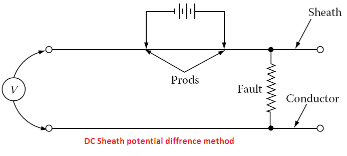
If the fault resistance is low enough or the internal resistance of the voltmeter is high enough, a voltage will be measured on the unfaulted side of the battery. Therefore, to locate the fault the battery contacts can be moved in the fault direction until the fault is located.
©yourelectricalguide.com/ underground cable fault location methods.