Thermocouple Working Principle & Types
RTDs are completely passive sensing elements, requiring the application of an externally-sourced electric current in order to function as temperature sensors.
Thermocouples, however, generate their own electric potential. In some ways, this makes thermocouple systems simpler because the device receiving the thermocouple’s signal does not have to supply electric power to the thermocouple.
It also makes thermocouple systems potentially safer than RTDs in applications where explosive compounds may exist in the atmosphere, because the power levels generated by a thermocouple tend to be less than the power levels dissipated by an RTD. The self-powering nature of thermocouples also means they do not suffer from the same “self-heating” effect as RTDs.
In other ways, however, thermocouple circuits are more complex and troublesome than RTD circuits because the generation of voltage actually occurs in two different locations within the circuit, not simply at the sensing point. This means the receiving circuit must “compensate” for temperature in another location in order to accurately measure temperature in the desired location.
Though typically not as accurate as RTDs, thermocouples are more rugged, have greater temperature measurement spans, and are easier to manufacture in different physical forms.
Dissimilar Metal Junctions
When two dissimilar metal wires are joined together at one end, a voltage is produced at the other end that is approximately proportional to temperature.
That is to say, the junction of two different metals behaves like a temperature-sensitive battery. This form of electrical temperature sensor is called a thermocouple.
This phenomenon provides us with a simple way to electrically infer temperature: simply measure the voltage produced by the junction, and you can tell the temperature of that junction.
And it would be that simple, if it were not for an unavoidable consequence of electric circuits: when we connect any kind of electrical instrument to the thermocouple wires, we inevitably produce another junction of dissimilar metals.
The following schematic shows this fact, where the iron-copper junction J1 is necessarily complemented by a second iron-copper junction J2 of opposing polarity:
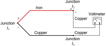
Junction J1 is a junction of iron and copper – two dissimilar metals – which will generate a voltage related to temperature. Note that junction J2, which is necessary for the simple fact that we must somehow connect our copper-wired voltmeter to the iron wire, is also a dissimilar-metal junction which will also generate a voltage related to temperature.
Further note how the polarity of junction J2 stands opposed to the polarity of junction J1 (iron = positive ; copper = negative). A third junction (J3) also exists between wires, but it is of no consequence because it is a junction of two identical metals which does not generate a temperature-dependent voltage at all.
The presence of this second voltage-generating junction (J2) helps explain why the voltmeter registers 0 volts when the entire system is at room temperature: any voltage generated by the ironcopper junctions will be equal in magnitude and opposite in polarity, resulting in a net (series-total) voltage of zero.
Only when the two junctions J1 and J2 are at different temperatures will the voltmeter register any voltage at all.
We may express this relationship mathematically as follows:
Vmeter = VJ1 − VJ2
With the measurement (J1) and reference (J2) junction voltages opposed to each other, the voltmeter only “sees” the difference between these two voltages.
Thus, thermocouple systems are fundamentally differential temperature sensors. That is, they provide an electrical output proportional to the difference in temperature between two different points.
For this reason, the wire junction we use to measure the temperature of interest is called the measurement junction while the other junction (which we cannot eliminate from the circuit) is called the reference junction (or the cold junction, because it is typically at a cooler temperature than the process measurement junction).
Much of the complexity of thermocouples is related to the reference junction voltage and how we must deal with that (unwanted) potential when using a thermocouple as a measuring device.
For most practical applications, we just want to measure the temperature at one location, not the difference in temperature between two locations which is what a thermocouple naturally does.
A number of different techniques exist to deal with this problem – forcing a differential temperature sensor to act like a single-point temperature sensor – and we will explore the most common techniques in this section.
Students and working professionals alike often find this concept of a reference junction and its effects endlessly confusing. My advice to the confused is to return to the simple iron-copper wire circuit shown previously as a “starting point,” and then deduce its behavior from first principles.
We know that a dissimilar-metal junction creates a voltage with temperature. We also know that in order to make a complete circuit with iron and copper wire there must be a second iron-copper junction somewhere else in that same circuit, the polarity of which is necessarily opposed to the first.
If we call the first iron-copper junction J1 and the second junction J2, we absolutely must conclude that the net voltage registered by the voltmeter in this circuit will be VJ1 − VJ2.
All thermocouple circuits – no matter how simple or complex – exhibit this fundamental property. Mentally constructing a simple circuit of two dissimilar-metal wires and then performing “thought experiments” to see how that circuit will behave with those junctions at the same temperature and also at different temperatures is the best way I can suggest for any person to comprehend thermocouples.
Students especially tend to cope with complexity through memorization: committing to memory catch-phrases and formulae such as Vmeter = VJ1−VJ2. This is a poor coping mechanism, as it grants the illusion of understanding with none of the substance.
The real secret is to know why a thermocouple circuit acts as it does, and that only comes through practiced reasoning.
In next article, as we explore reference junction compensation, how to interpret voltage measurements in thermocouple circuits, and how to simulate thermocouples at temperature, we will keep returning to this simple iron-copper wire circuit to refresh our understanding of how and why thermocouple circuits behave.
If you understand this one fundamental concept, the rest will make sense to you. If you continually find yourself confused by thermocouple circuits, it means you do not yet fully understand this basic circuit, and you need to return to it and think it through until you do.
Thermocouple Types
Thermocouples exist in many different types, each with its own color codes for the dissimilar-metal wires. Here is a table showing the more common thermocouple types and their standardized colors (the colors in this table apply only to the United States and Canada.), along with some distinguishing characteristics of the metal types to aid in polarity identification when the wire colors are not clearly visible:
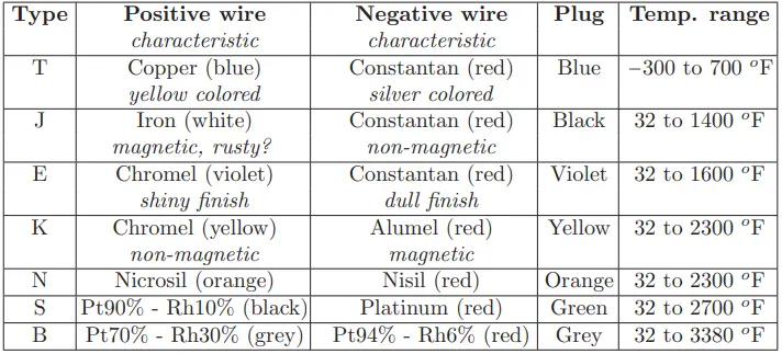
Types S and B use platinum or platinum-rhodium alloy wire, with different alloying distinguishing the positive from the negative wires. Sometimes type B is colored green and red rather than grey and red.
Note how the negative (−) wire of every thermocouple type is color-coded red. While this may seem backward to those familiar with modern electronics (where red and black usually represent the positive and negative poles of a DC power supply, respectively), bear in mind that thermocouple color codes actually pre-date electronic power supply wire coloring!
Aside from having different usable temperature ranges, these thermocouple types also differ in terms of the atmospheres they may withstand at elevated temperatures.
- Type J thermocouples, for instance, by virtue of the fact that one of the wire types is iron, will rapidly corrode in any oxidizing atmosphere.
- Type K thermocouples are attacked by reducing atmospheres as well as sulfur and cyanide.
- Type T thermocouples are limited in upper temperature by the oxidation of copper (a very reactive metal when hot), but stand up to both oxidizing and reducing atmospheres quite well at lower temperatures, even when wet.
One final note on the thermocouple types shown in this table is that the temperature ranges given are approximate, and vary with the intended measurement accuracy.
One may have to stay within a more limited range of temperature than what is shown in this table if a certain minimum level of accuracy is desired from the thermocouple. Consult manufacturers’ data for details!
Thermocouple Connector and Tip Styles
In its simplest form, a thermocouple is nothing more than a pair of dissimilar-metal wires joined together. However, in industrial practice, we often must package thermocouples in a more rugged form than a bare metal junction.
For instance, most industrial thermocouples are manufactured in such a way that the dissimilar-metal wires are protected from physical damage by a stainless steel or ceramic sheath, and they are often equipped with molded-plastic plugs for quick connection to and disconnection from a thermocouple-based instrument.
Thermocouple wires are most often manufactured in solid form rather than stranded form. A common mistake made with thermocouple wires is for technicians to crimp compression-style terminals (“lugs”) onto the solid wires.
While this may form a usable connection at first, compression-style terminals are simply unable to maintain adequate compression when applied to solid wire of any type, thermocouple wire included. Over time, solid wires will loosen inside compression terminals leading to circuit problems.
In the case of a thermocouple circuit, bad wire connections lead to a situation where the receiving instrument “thinks” the thermocouple has failed open. This situation is commonly called burnout, referring to the phenomenon where a thermocouple junction fails open from being “burned out” by excessive temperature.
You will most often find compression terminals (improperly) applied to solid thermocouple wire tips where those wires must terminate under the head of a screw.
Compression terminals are correct to use in applications where stranded wire terminates at a screw head, but not solid wire. The proper termination technique for solid wire under a screw head is to wrap the solid wire in a semi-circle and directly clamp it under the screw head. At the other end of the thermocouple, we have a choice of tip styles.
For maximum sensitivity and fastest response, the dissimilar-metal junction may be unsheathed (bare). This design, however, makes the thermocouple more fragile.
Sheathed tips are typical for industrial applications, available in either grounded or ungrounded forms:
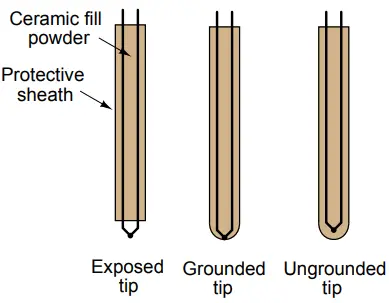
Grounded-tip thermocouples exhibit faster response times and greater sensitivity than ungrounded-tip thermocouples, but they are vulnerable to ground loops: circuitous paths for electric current between the conductive sheath of the thermocouple and some other point in the thermocouple circuit.
In order to avoid this potentially troublesome effect, most industrial thermocouples are of the ungrounded design.
Manually Interpreting Thermocouple Voltages
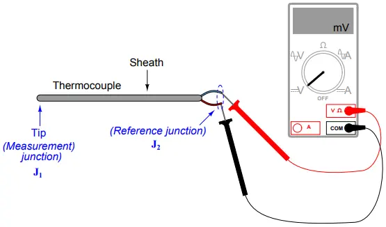
Recall that the amount of voltage indicated by a voltmeter connected to a thermocouple is the difference between the voltage produced by the measurement junction (the point where the two dissimilar metals join at the location we desire to sense temperature at) and the voltage produced by the reference junction (the point where the thermocouple wires join to the voltmeter wires):
This makes thermocouples inherently differential sensing devices: they generate a measurable voltage in proportion to the difference in temperature between two locations. This inescapable fact of thermocouple circuits complicates the task of interpreting any voltage measurement obtained from a thermocouple.
In order to translate a voltage measurement produced by a voltmeter connected to a thermocouple, we must add the voltage produced by the measurement junction (VJ2) to the voltage indicated by the voltmeter to find the voltage being produced by the measurement junction (VJ1).
In other words, we manipulate the previous equation into the following form: VJ1 = VJ2 + Vmeter
We may ascertain the reference junction voltage by placing a thermometer near that junction (where the thermocouple wire attaches to the voltmeter test leads) and referencing a thermocouple table showing temperatures and corresponding voltages for that thermocouple type.
Then, we may take the voltage sum for VJ1 and re-reference that same table, finding the temperature value corresponding to the calculated measurement junction voltage.
The National Institute of Standards and Technology (NIST) in the United States publishes tables showing junction voltages and temperatures for standardized thermocouple types.
While it is possible to mathematically model a thermocouple junction’s voltage in the same way we may model an RTD’s resistance, the functions for thermocouples are less linear than for RTDs, and so tables are greatly preferred for practical use.
To illustrate, suppose we connected a voltmeter to a type K thermocouple and measured 14.30 millivolts. A thermometer situated near the thermocouple wire / voltmeter junction point shows an ambient temperature of 73 degrees Fahrenheit.
Referencing a table of voltages for type K thermocouples (in this case, the NIST “ITS-90” reference standard), we see that a type K junction at 73 degrees Fahrenheit corresponds to 0.910 millivolts.
Adding this figure to our meter measurement of 14.30 millivolts, we arrive at a sum of 15.21 millivolts for the measurement (“hot”) junction.
Going back to the same table of values, we see 15.21 millivolts falls between 701 and 702 degrees Fahrenheit. Linearly interpolating between the table values (15.203 mV at 701 oF and 15.226 mV at 702 oF), we may more precisely determine the measurement junction to be 701.3 degrees Fahrenheit.
The process of manually taking voltage measurements, referencing a table of millivoltage values, performing addition, then re-referencing the same table is rather tedious.
Compensation for the reference junction’s inevitable presence in the thermocouple circuit is something we must do, but it is not something that must always be done by a human being.
The next article discusses ways to automatically compensate for the effect of the reference junction, which is the only practical alternative for continuous thermocouple-based temperature instruments.