Hysteresis and eddy current losses together constitute the no-load loss according to the classical theory. The loss due to the no-load current flowing in the primary winding is negligible.
Also, at the rated flux density condition on no-load, since most of the flux is confined to the core, negligible losses are produced in the structural parts due to near absence of stray flux.
The hysteresis and eddy losses arise due to successive reversals of the magnetization in the iron core excited by a sinusoidal voltage source at a particular frequency f (cycles/second).
The eddy loss, occurring on account of eddy currents produced due to induced voltages in laminations in response to an alternating flux, is proportional to the square of the thickness of laminations, the square of the frequency and the square of the effective (r.m.s.) value of the flux density.
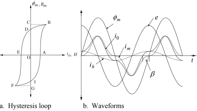
The hysteresis loss is proportional to the area of the hysteresis loop; a typical loop is shown in Figure 1(a).
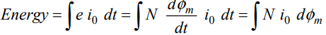
Let e , io and ɸm denote the induced voltage, the no-load current and the core flux, respectively. The e leads ɸm by 90°. Due to the hysteresis phenomenon, io leads ɸm by the hysteresis angle (β) as shown in Figure 1(b).
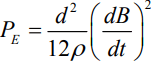
Energy, either supplied to the magnetic circuit or returned back by the magnetic circuit, is given by
If we consider the first quadrant of the hysteresis loop, the area OABCDO represents the supplied energy.
The induced voltage and the current are positive for path AB. For path BD, the energy represented by the area BCD is returned to the source since the two quantities are having opposite signs giving a negative value of energy.
Thus, the area OABDO represents the energy loss in the first quadrant, whereas the area ABDEFIA represents the total hysteresis loss in one cycle.
The loss has a constant value per cycle meaning thereby that it is directly proportional to frequency; the higher the frequency, the higher the loss is.
The non-sinusoidal current, io, can be resolved into two components: im and ih . The ih component, which is in phase with e, represents the hysteresis loss, and im is the non-sinusoidal magnetizing component. The eddy loss ( Peddy ) and the hysteresis loss ( Physteresis ) are given by
Peddy = k1 f2 t2 B2rms (Equation 2)
Physteresis = k2 f Bnmp (Equation 3)
Where t is the thickness of the core laminations; k1 and k2 are constants which are material dependent; Brms is the rated effective flux density corresponding to the actual r.m.s. voltage on the sine wave basis; Bmp is the actual peak value of the flux density; n is the Steinmetz constant having a value of 1.6 to 2.0 for hot-rolled laminations and a value of more than 2.0 for cold-rolled laminations due to the use of higher operating flux density in them.
In r.m.s. notations, when the hysteresis loss component (Ih) shown in Figure 1(b) is added to the eddy loss component, we get the total core loss current ( Ic ).
In practice, Equations 2 and 3 are not used by designers for calculation of the no-load loss. There are at least two approaches generally used; based on test results/experimental data, either the building factor of the entire core is determined or an empirical factor is derived for accounting the effect of the weight at the joints separately:
No load loss = Wt x Kb x w (Equation 4)
or No load loss = (Wt – Wc ) x w + Wc x w x Kc (Equation 5)
Where, w is watts/kg for a particular operating peak flux density as given by the supplier (Epstein core loss for a single lamination), Kb is the building factor, Wc denotes the weight of the joints out of the total weight of Wt , and Kc represents the extra loss occurring at the joints (whose value is higher for smaller core diameters).
Inclusion of Anomalous Loss
As discussed earlier, the core loss in transformers is usually classified into two components, viz. the eddy loss and the hysteresis loss, according to the classical theory. The hysteresis loss is due to the irreversible nature of the magnetic characteristics (B-H curves) when H is repeatedly cycled between –Hm to +Hm as explained earlier.
The eddy loss arises due to induced voltages on account of a changing magnetic induction B; the voltages lead to currents circulating in closed loops. These eddy currents cause a resistive loss.
The core losses can be calculated by simple formulae given by Equations 2 and 3 which assume a non-domain structure of the material. They also assume sinusoidal variation of B. Therefore, the classical theory tends to underestimate the core loss.
The difference between the measured core loss and the calculated hysteresis loss is the apparent eddy loss, and the difference between the apparent and classical eddy loss values is the anomalous loss.
In the grain oriented transformer steel under normal working conditions, the anomalous loss can be about one-half of the total core loss.
Many efforts have been made in the literature for describing the three components of the core loss using a theory based on magnetic domains. A change in magnetization of the core material occurs because of the motion of the domain walls and the rotation of the domain magnetization.
The hysteresis loss is caused by the resistance to the domain wall motion due to defects (impurities or dislocations in crystallographic structure) and internal strains in the material.
Hysteresis loss: This loss corresponds to the area enclosed by the DC hysteresis loop. It represents the energy expenditure per cycle of the loop as discussed earlier. Imperfections in the material cause an increase in the energy expenditure during the magnetization process, in the form of a kind of internal friction to the domain wall motion.
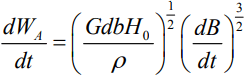
Eddy losses: The eddy loss in a lamination can be calculated using the classical theory which assumes uniform flux throughout its thickness. According to the theory, the instantaneous eddy loss per unit volume is expressed in terms of the rms value of the flux density (B) as
Where d indicates the thickness of a single lamination and ρ is the resistivity of its material. When the magnetic induction B is sinusoidally varying, d/dt is replaced by jω and the above expression becomes numerically equal to B = Bo/√2 ,
PE = ke (f Bo)2 (Equation 7)
Where, ke = π2d2 / (6ρ).
The above expression is of the same form as Equation 2. Thus, the classical eddy currents are proportional to the square of the thickness of the lamination and to the square of the frequency of supply. The loss is inversely proportional to resistivity of the material.
Anomalous loss or microscopic eddy current loss: The measured power losses for ferromagnetic materials are usually two or three times the value calculated by using the classical eddy current theory. This problem is referred to as the eddy current anomaly.
Several attempts to explain this anomaly are based on non-uniform magnetization in the core materials due to the presence of magnetic domains. A model has been frequently used in the literature for interpreting anomalous losses. It assumes an infinite lamination containing a periodic array of longitudinal domains and calculates the eddy current loss using Maxwell’s equations.
The model gives an excess loss in terms of microscopic eddy currents associated with the domain wall motion. The discrepancies between the losses given by the model and measurements have been related to effects such as the presence of irregularities in the wall motion, domain multiplications, and wall bowing.
A statistical approach has been found to give reasonably accurate results. The anomalous loss results from the domain wall motion, which can be expressed as
Where, G is a dimensionless coefficient representing a damping effect of the
eddy currents (0.136), b indicates the width of the lamination, and d and ρ
represent the thickness and resistivity of the lamination, respectively. H0 characterizes the statistical distribution of the internal domain wall field and takes into account the grain size.
It should be noted that this formula will give inaccurate results if the skin effect is not negligible. For electrically thick (i.e., the thickness is much greater than the skin depth) sheets, the formula does not hold.