In many situations, the raw output of the sensor may not be in a form suitable to be interfaced to a measurement device or an A/D convertor, and some form of signal conditioning is needed to be applied to the sensor output. These signal conditioning operations include filtering, amplification, or using a bridge circuit.
In dynamic measurements, the output of a sensor or a transducer consists of many frequency components. The output can also be corrupted with noise. The noise can be from external disturbances such as heat or vibration, imperfections in the sensor component materials, or from external signal interference. The noise reduces the sensor resolution and worsens the repeatability error.
Filtering is the process of attenuating unwanted components or noise from the sensor output and allowing other components to pass.
Signal Conditioning by Filter Circuits
We will discuss different types of filter circuits. These include low-pass, high-pass, notch, and band-pass. The naming of these filters is in reference to desired frequency characteristics of the filter.
A filter can be implemented using analog circuit components such as op-amps and capacitors and is thus referred to as an analog filter, or using computer code in a digital signal processer chip and thus referred to as a digital filter.
Digital filters offer flexibility over analog filters since changing the filter characteristics involves only code change. However, analog filters are inexpensive and more robust.
Analog filters can be classified as passive or active. A passive filter does not require any external power to operate. An example of a passive analog filter is the first-order RC-circuit filter.
An active filter, on the other hand, requires external power to operate. Active filters use components such as op-amps.
The filtering action is best described using frequency response plots and transfer function concepts. A frequency response plot shows the output–input relationship for the filter as a function of frequency. The plot has two components: magnitude and phase. The magnitude is the ratio of the output signal to the input signal, while the phase is the time shift between the output and the input signals.
A positive phase angle means that the output signal leads the input signal, while a negative phase shift means that the output signal lags the input signal. The magnitude plot is normally shown in units of dB, where 1 dB 20 log10(output/input).
frequency response characteristics of
various filters.
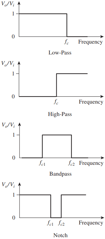
The ideal magnitude frequency response characteristics for the low-pass, high-pass, band-pass, and notch filters are shown in Figure 1, where fc is the filter corner frequency.
The figure shows that over the frequencies at which the filtering is active the output signal is zero. In reality, these ideal frequency characteristics cannot be achieved.
First, filters with zero passing are difficult to construct. Second, the sharp transitions shown in the figure cannot be achieved.
Low-Pass Filter Circuits
Low-pass filters are used to attenuate frequency signals above the corner frequency fc such as the 60-Hz interference signals from AC power operated equipment. These filters are commonly used to process signals from tachometer and temperature sensors.
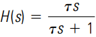
There are many forms of low-pass filters, so we will restrict our discussion to the first-order, low-pass filter given by the transfer function
where τ is the time constant of the filter.
The time constant τ in seconds and the corner frequency fc in Hz are related by
fc = 1/2πτ
The order of the filter refers to the highest power in the denominator of the filter transfer function. A first-order filter is also known as a single-pole filter, since the characteristic equation of the filter has only one pole or one root.

The magnitude and phase frequency response plots of this filter are shown in Figure 2. The magnitude plot shows that the filter output-to-input magnitude has a unity gain before the corner frequency at ωc, where (ωc = 1/τ ), but the gain decreases slowly as the frequency approaches the corner frequency.
At the corner frequency, the output magnitude is -3dB with the output at 70.7% of the input. After the corner frequency, the magnitude starts dropping much faster at the rate of 20 dB/decade, where a decade means a factor of 10 increase or decrease in the frequency.
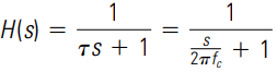
A simple passive low-pass filter can be easily constructed using a resistor and a capacitor circuit as shown in Figure 3(a). The filter time constant τ is the product of the resistance and the capacitance or τ = RC.
low-pass RC filter and (b) active low-pass filter.
An active low-pass filter is implemented using op-amps as shown in Figure 3(b), where the filter time constant τ is given as R2C. Note for the active filter, the filter gain is given by (–R2/R1).
The attenuation rate of the first-order low-pass-filter is, however, not high. It is desirable to have high attenuation rates such as 60 dB/decade. Such an attenuation rate can be achieved by other types of filters such as Butterworth and Chebyshev.
If the sensor data is available digitally, then one can use a digital filter instead. A digital low-pass filter can be implemented using the folloing Equation
y(k) = (1 – α)x(k) + αy(k – 1)
Where y(k) is the output sequence, x(k) is the input sequence, k is the current index, and α is a factor that is dependent on the filter corner frequency fc and the sampling time T. Alpha is given by: α = e(-2 πfcT )
For example, if fc = 10Hz, and T is 1 ms, then α is 0.9391, and the digital filter equation is
y(k) = 0.0609x(k) + 0.9391y(k – 1)
The above iterative equation can be easily implemented in code using a For-Loop or similar construct.
different corner frequencies.
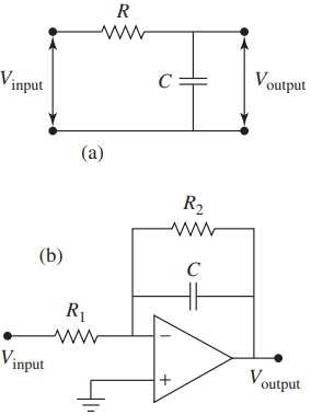
Figure 4 shows the filter output for a 10 Hz sinusoidal input signal for three corner frequencies: 1, 5, and 10 Hz and a sampling time of 1 ms. Notice how the output magnitude is smaller than the input magnitude for all the three cases.
High-pass Filter Circuits
High-pass filters are used to attenuate frequency signals below the corner frequency, fc. These filters are used to attenuate dc and low-frequency components from a signal so the high-frequency components of the signal become more distinguished.
Similar to the low-pass case, there are many forms of high-pass filters, so we will restrict our discussion to the first-order, high-pass filter given by the transfer function
Where τ is the time constant of the filter. The magnitude and phase frequency response plots of this filter are shown in Figure 5, and they are opposite to those of the low-pass filter. The plot shows that the filter has nearly a unity gain above the corner frequency ωc. Before this frequency, the magnitude increases at the rate of 20 dB/decade.
high-pass filter
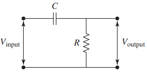
A simple high-pass filter can also be constructed using a resistor and capacitor circuit as shown in Figure 6. The circuit is similar to the low-pass filter, but the resistor and the capacitor locations are interchanged. Bandpass filters are used to allow signals in a certain frequency range and to attenuate all signals outside of this range.
The two corner frequencies that define this frequency range are fcl and fch. A bandpass filter is a cascade combination of a low-pass and a high-pass filter, with the transfer function given as
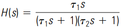
Where τ1 = 1/(2πfcl) = 1/ωcl and τ2 = 1/(2πfcl) = 1/ωcl.
The magnitude and phase frequency response plots of this filter are shown in Figure 7.
The magnitude plot shows that the filter has nearly a unity gain inside the desired frequency band. Outside this band, the magnitude increases or drops at the rate of 20 dB/decade. The phase angle is close to zero around the center of the pass band, but approaches 90 degrees away from the frequency band.
Notch Filter Circuits
Notch filters are used to attenuate a narrow band of frequencies from a signal. For example, if we know that the noise is originating at a particular frequency such as 60 Hz, then we can design a filter to eliminate this noise. A notch filter is a second-order system and has the following transfer function:
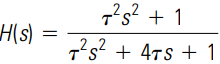
Where, as before, τ the time constant and the notch frequency fc are related by Equation (7.37).
The magnitude and phase frequency response plots of this filter are shown in Figure 8.
The magnitude plot shows that the filter has zero output at the notch frequency (10 rad/s), with a sharp roll down and roll up at either side of the notch frequency.
The phase plot shows that away from the notch frequency, the phase angle is zero. Note that if the disturbance frequency is different from fc, then the disturbance frequency is not completely eliminated.