Applications of Functional Model

A representative T/X sketch, Figure 1, for a dual-reference junction thermocouple with two extensions, Figure 2, illustrates T/X application. It shows one deliberately inappropriate yet plausible temperature distribution.

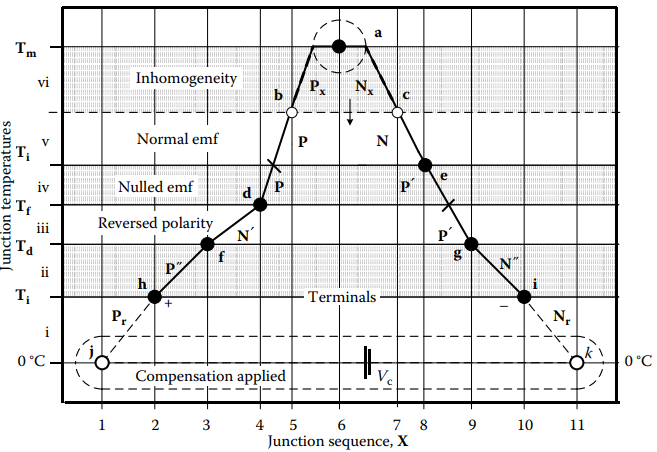
It reveals how particular segments of thermoelements, variably, are thermally paired in electrical effect, with different segments that may be remote in the circuit. It also illustrates the commonplace profound effect of unrecognized inhomogeneity in thermometry.

The T/X sketch, applied here to the two basic thermocouple circuits, depicts the significant circuit elements (the junctions and thermoelements) in a way that focuses on their temperature-determined thermoelectric functions (Corollaries 1 and 2). The T/X sketch illustrates realistic, commonplace, yet usually unrecognized, problems of circuits used in thermometry.

For illustration, circuits are here depicted with plausible defects or with improperly controlled incidental junction relative temperatures. Each kind of error source represented here has been recognized as significant in practical application and even in calibration performed by qualified calibration laboratories.

The errors, if not detected, would have significantly degraded thermometry and invalidated costly calibrations. Viewed from the perspective of the spurious junction source model, the thermal response of such circuits sometimes has been very puzzling.

Note: Though usually hidden, most such commonplace problems are easily recognized, diagnosed, and avoided if thermoelectric principles are understood and applied.

Dual-Reference-Junction Circuit

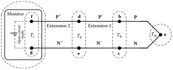
Figure 1 is a T/X sketch for an initially homogeneous then use-degraded dual-reference junction thermocouple, Figure 2, with measuring thermocouple PN, junctions d and e, and two extensions P′N′ and P″N″. This single T/X sketch illustrates eight of the commonplace obscure sources of error additional to any calibration, instrument, or thermal coupling error. One or more of these, or other such errors, can occur in any installation.

Temperature Zones i through vi each contribute essential Seebeck emf. Zone ii shows the corresponding-type extension in appropriate polarity, but Zone iii has the extension, N′P′, in reversed polarity. (Zone ii might have been improperly of a passive-type extension.) Zone iv thermally pairs very similar segments, P and P′, inappropriately contributing too little emf.

Note that if T_d is greater than T_e, the emf from Zone iv is from a very different thermoelement pair.

Inhomogeneous Segments: Troublesome inhomogeneity most often occurs around a severely heated measuring junction. Severe damage, experienced as drift, often is not visible on the thermoelements nor recognized as inhomogeneity in thermometry. Figure 1 shows measuring junction, a, with adjoining segments of thermoelements appropriately immersed within an isothermal region (as in calibration.)

However, heat-damaged segments, P_x and N_x, extend from junction a to phantom real junctions b and c that bound the damage. This portion of the inhomogeneity, as in calibration, lies partially in the isothermal zone at junction a, where it contributes no emf, but it extends to a location of much lower temperature, T_x. (Realistically, the degradation would affect the dissimilar thermoelements differently so b and c would not likely be isothermal.)

In thermometry, this damage usually spans the highest temperature zone where the effect of its modified emf is greatest in thermometry. (When inhomogeneity is hidden isothermally, recalibration is invalidated.)

Electrical Shorting: Note that mechanical damage apart from the junction could incidentally result in a progressive contact short junction between legs, as directly between b and c. That would result in uninterrupted temperature indication from a different location along the thermoelements and probably at a different local temperature than the perceived measuring junction with no definite warning of serious thermocouple failure.

Compensation Scaling Error: This T/X sketch illustrates the contribution of reference junction temperature compensation, when needed, by virtual thermoelements P_r and N_r. The compensation characteristic, which only approximates the standard Seebeck characteristic, is at least slightly different from the one used for scaling the thermocouple emf.

Scaling error in this temperature zone can be substantial yet remain unnoticed. That reference affects scaling at all temperatures. Some approximations initially are, or else progressively become, inaccurate.

Inappropriate Reference Temperature Compensation: Compensation error is usually unrecognized even if it is significant and variable. It can occur

1. due to lack of needed compensation,
2. as redundant compensation at more than one set of reference junctions,
3. as compensation applied to junctions inappropriate for the extension style, or
4. simply of incorrect value.

A similar magnitude of error occurs whether no compensation is applied or whether proper compensation is applied, but redundantly at two sets of reference junctions.

Compensation at the Monitor: Typical thermocouple monitors apply compensation voltage at input terminal junctions h and i. That reference temperature compensation feature should be selectable because compensation sometimes must not be applied there. Compensation must be at the monitor terminals for the basic measuring thermocouple PN alone or else with complete corresponding- or compensating-type extensions, P′N′, and so on. It must not be at the monitor if passive extensions are used.

Compensation Apart from the Monitor: If all extensions are of the passive style, reference temperature compensation must be applied only at terminal junctions d and e external to the monitor and not also or alternatively at the monitor.

If T_i and T_d are similar and compensation is improperly applied at the monitor, the error might be small but significant and variable and remain unrecognized.

However, if the transition from the measuring thermocouple to extensions is remote from the monitor, those junction temperatures could be very different and the error significant but inconspicuous relative to the indicated temperature.

Compensation with Multiple Extensions: Each extension interface risks introduction of thermoelements that might accidentally be of slightly or very different material types, of incorrect style, or else be connected in crossed polarity as by misinterpretation of color codes.

Each extension connection introduces incidental junctions. In such instances, the compensation could be misplaced at the measuring thermocouple, at the monitor, between a corresponding-style extension and a passive-style extension, and so on.

Reversed Polarity: Error resulting from polarity reversal of extensions may not be recognized even if it is significant. Misunderstood or contradictory polarity color codes risk accidentally connecting extensions in reversed polarity at d and e or at f and g so that the extension, unnoticed, effectively becomes relatively an N′P′ pairing in the circuit, Zone iii.

If temperatures of incidental extension junctions are different, polarity reversal at either end of extension P′N′ introduces error. Also if an obvious polarity error is noticed in temperature indication and polarity then is merely reversed at the monitor or measuring thermocouple, a different error is introduced.

If dissimilar thermoelements are spliced, hidden within insulators or connector shells, along the circuit, the hidden incidental junction can be found with a swept “temperature spike” test.

Single-Reference-Junction Circuit

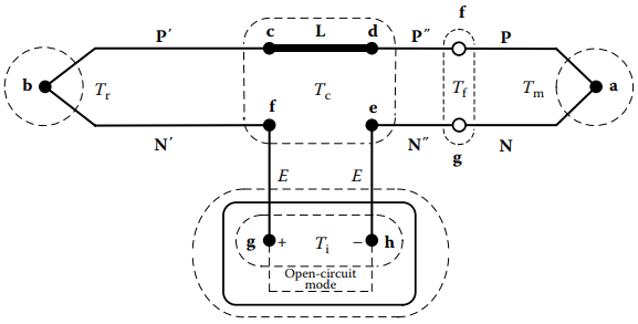
This commonplace circuit, Figure 3, is widely used for convenience in routine calibration of a measuring thermocouple, PN, as well as for thermometry. Represented by a T/X sketch, Figure 4, plausible error sources are introduced for illustration. The monitor must not apply electronic compensation for this circuit inappropriately as is shown in the sketch.

Reference Thermocouple: The reference thermocouple, P′N′, of the same nominal type as the measuring thermocouple, usually is separately purchased as an assembly with thermocouple connectors and passive-type extension leads, E, that contribute no net emf in Zone iv as they are of the same type. Except for use in thermocouple type-characterization, they are of a type different from N. Usually they are of copper.

The measuring thermocouple, PN, with optional extension P″N″, plugs into the jack of the reference thermocouple assembly at points d and e. Reference junction, b, should be held accurately at reference temperature, 0°C but is shown at slightly higher temperature.

However, as this reference thermocouple is separately fabricated and purchased, reference junction thermocouple, P′N′, has a Seebeck characteristic that, even if within tolerance, is different from the PN thermocouple. Typically, it is not individually calibrated.

As T_b and T_f are very different, when the measuring junction temperature is near ambient, all or most of an observed “calibration” emf is from the uncalibrated reference thermocouple even with proper isothermal temperature control of link L. Calibration of PN is compromised at all temperatures. This systematic reference error source should be acknowledged in a calibration report, but it can neither be eliminated nor corrected.

Incidental Junctions: The connector components, ideally isothermal in Zone iii, and the monitor input terminals separately are to be isothermal at temperatures that should both be near ambient temperature. Just as in the dual reference junction circuit, the temperatures of incidental junctions must be controlled. For illustration of error source, they are shown uncontrolled in the T/X sketch (Figure 4).

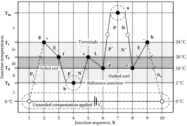
Such incidental errors often are not evident in calibration or in temperature indications, even if they are significant. Fortunately, most of the hidden error sources illustrated in Figures 70.5 and 70.6 are very easily avoided, but only if recognized.

Avoidance of most errors by isothermal control of incidental junctions using passive thermal lagging and insulation usually is very easy. A practical significance of the T/X schematic is that it forces the attention to specific incidental junctions of which temperatures must be controlled to avoid hidden error. It also guides estimate of plausible error.

Paralleled Thermoelements

In some situations, two or more thermoelements might accidentally be paralleled by electrical contact at widely separate points that are at different temperatures as by multiple shorting of a shield to thermoelements or between multiple thermoelements within a mineral-insulated, metal-sheathed (MIMS) thermocouple.

Alternatively, by design, legs of dissimilar paralleled thermoelements have been used as a compound leg, intending to make a leg of customizable relative Seebeck coefficient. Figure 5 shows a circuit with a negative leg paralleled to form a loop by T/X sketch. The overall circuit is monitored in the usual “open-circuit” mode, but it includes a closed loop that locally results in current that affects the net voltage.

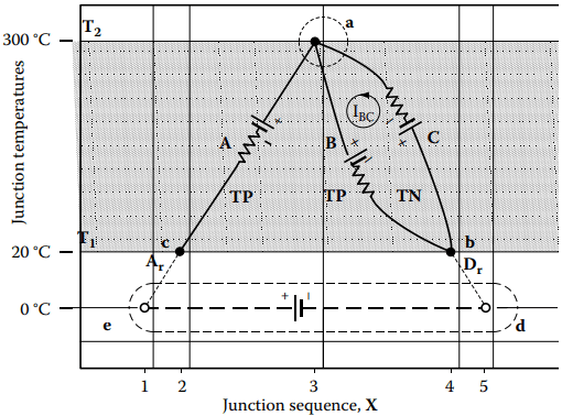
The net loop voltage is affected by temperature-dependent resistance, therefore, by wire diameter and thermoelement lengths. Thus, the effective Seebeck coefficient of the paralleled leg is not a function of junction temperature alone as it must be for thermometry. This is a source of error. The paralleled leg circuit is inappropriate for accurate thermometry but occurs as a defect.

Just for illustration, let thermoelement legs A and B both be of Type TP and leg C of Type TN. Values for these thermoelements relative to Pt-67 are tabulated by NIST. Resistances of 3 Ft., 22 AWG, legs A and B are 0.0483 Ω. Leg C resistance is, 1.728 Ω.

Between junction temperatures 20 and 300 °C, relative to a shared Pt-67 reference, Seebeck emfs for the TP legs would be 3,024.0 μV. Leg C alone would contribute 11,048.4 μV. The Seebeck emf would result in a loop current of 4.517 mA reducing the net loop voltage to 3242.1 μV.

As a normal “open-circuit” TP/TN thermocouple, an AB pair alone would contribute 14,072.4 μV. Seebeck emf-induced current has reduced the net emf voltage by 10,830.3 μV.

Note: The BC loop is a closed-circuit “thermocouple” as employed by Seebeck.

• Thermocouple Working Principle
• Absolute Seebeck Effect
• Basic Thermocouple Circuits
• Extensions of Thermocouple
• Functional Model of Thermoelectric Circuits
• T/X Sketch of Dual-Reference Junction Circuit
• Applications of Functional Model
• Characteristics of Thermocouples
• Thermocouple Hardware
• Thermocouple Junction Styles
• Active Tests of Thermocouple
• Calibration of Thermocouples
• Thermocouple Thermometry Practice
• Distinctive Thermocouple Noise Problems