PLC Data Manipulation Programs
Data manipulation instructions give new dimension and flexibility to the programming of control circuits. For example, consider the hardwired relay-operated, time-delay circuit in Figure 1 .
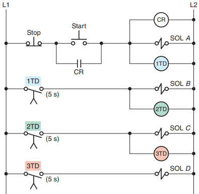
This circuit uses three electro-mechanical time-delay relays to control four solenoid valves. The operation of the hardwired circuit can be summarized as follows:
- When the momentary start pushbutton is pressed solenoid A is energized immediately.
- Solenoid B is energized 5 s later than solenoid A.
- Solenoid C is energized 10 s later than solenoid A.
- Solenoid D is energized 15 s later than solenoid A.
The hardwired time-delay circuit could be implemented using a conventional PLC program and three internal timers. However, the same circuit can be programmed using only one internal timer along with data compare instructions.

Figure 2 shows the program required to implement the circuit using only one internal timer. The operation of the program can be summarized as follows:
- The momentary stop button is closed.
- When the momentary start button is pressed, SOL A output energizes immediately to switch on solenoid A.
- SOL A examine-on contact becomes true to seal in output SOL A and to start on-delay timer T4:1 timing.
- The timer preset time is set to 15 seconds.
- Output SOL D will energize (through the timer done bit T4:1/DN) after a total time delay of 15 seconds to energize solenoid D.
- Output SOL B will energize after a total time delay of 5 seconds, when the accumulated time becomes equal to and then greater than 5 seconds. This, in turn, will energize solenoid B.
- Output SOL C will energize after a total time delay of 10 seconds, when the accumulated time becomes equal to and then greater than 10 seconds. This, in turn, will energize solenoid C.

Figure 3 shows an application of an on-delay timer program implemented using the EQU instruction. The operation of the program can be summarized as follows:
- When the switch (S1) is closed, timer T4:1 will begin timing.
- Both EQU instructions’ source A s are addressed to get the accumulated value from the timer while it is running.
- The EQU instruction of rung 2 has the value of 5 stored in source B.
- When the accumulated value of the timer reaches 5, the EQU instruction of rung 2 will become logic true for 1 second.
- As a result, the latch output will energize to switch the pilot light PL1 on.
- When the accumulated value of the timer reaches 15, the EQU instruction of rung 3 will be true for 1 second.
- As a result, the unlatch output will energize to switch the pilot light PL1 off.
- Therefore, when the switch is closed, the pilot light will come on after 5 seconds, stay on for 10 seconds, and then turn off.
PLC Data Manipulation Programs

Figure 4 shows an application of an up-counter program implemented using the LES instruction. The operation of the program can be summarized as follows:
- Up-counter C5:1 will increment by 1 for every false-to-true transition of the proximity sensor switch.
- Source A of the LES instruction is addressed to the accumulated value of the counter and source B has a constant value of 20.
- The LES instruction will be true as the long as the value contained in source A is less than that of source B.
- Therefore, output solenoid SOL will be energized when the accumulated value of the counter is between 0 and 19.
- When the counter’s accumulated value reaches 20, the LES instruction will go false, de-energizing output solenoid SOL.
- When the counter’s accumulated value reaches its preset value of 50, the counter reset will be energized through the counter done bit (C5:1/DN) to reset the accumulated count to 0.
The use of comparison instructions is generally straightforward. However, one precaution involves the use of these instructions in PLC programs used to control the flow in vessel filling operations. This control scenario can be summarized as follows:
- The receiving vessel has its weight monitored continuously by the PLC program as it fills.
- When the weight reaches a preset value, the flow is cut off.
- While the vessel fills, the PLC performs a comparison between the vessel’s current weight and a predetermined constant programmed in the processor.
- If the programmer uses only the equal instruction, problems may result.
- As the vessel fills, the comparison for equality will be false. At the instant the vessel weight reaches the desired preset value of the equal instruction, the instruction becomes true and the flow is stopped.
- However, should the supply system leak additional material into the vessel, the total weight of the material could rise above the preset value, causing the instruction to go false and the vessel to overfill.
- The simplest solution to this problem is to program the comparison instruction as a greater than or equal to instruction. This way, any excess material entering the vessel will not affect the filling operation.
- It may be necessary, however, to include additional programming to indicate a serious overfill condition.
Numerical Data I/O Interfaces
The expanding data manipulation processing capabilities of PLCs led to the development of I/O interfaces known as numerical data I/O interfaces. In general, numerical data I/O interfaces can be divided into two groups: those that provide interface to multibit digital devices and those that provide interface to analog devices. The multibit digital devices are like the discrete I/O because processed signals are discrete (on/off).
The difference is that, with the discrete I/O, only a single bit is required to read an input or control an output. Multibit interfaces allow a group of bits to be input or output as a unit. They can be used to accommodate devices that require BCD inputs or outputs.

The thumbwheel switches (TWS), shown in Figure 5, are typical BCD input devices. Each one of the four switches provides four binary digits at its output that correspond to the decimal number selected on the switch. The conversion from a single decimal digit to four binary digits is performed by the TWS device.
The BCD input module allows the processor to accept the 4-bit digital codes and input their data into specific register or word locations in memory to be used by the control program. Data manipulation instructions can be used to access the data from the input module allowing a person to change set points, timer, or counter presets externally without modifying the control program.

The seven-segment LED display board, shown in Figure 6, is a typical Binary Coded Decimal (BCD) output device. It displays a decimal number that corresponds to the BCD value it receives at its input. Conversion of the four binary bits to a single decimal digit on the display is performed by the LED display device.
The BCD output module is used to output data from a specific register or word location in memory. This type of output module enables a PLC to operate devices that require BCD coded signals.

Figure 7 shows a PLC program that uses a BCD input interface module connected to a thumbwheel switch and a BCD output interface module connected to an LED display board. The program is designed so that the LEDs display the setting of the thumbwheel switch. Both the MOV and EQU instructions form part of the program. The operation of the program can be summarized as follows:
- The LED display board monitors the decimal setting of the thumbwheel switch.
- The MOV instruction is used to move the data from the thumbwheel switch input to the LED display output.
- Setting of the thumbwheel switch is compared to the reference number 1208 stored in source B by the EQU instruction.
- Pilot light output PL is energized whenever the input switch S1 is true (closed) and the value of the thumbwheel switch is equal to 1208.
Input and output modules can be addressed either at the bit level or at the word level. Analog modules convert analog signals to 16-bit digital signals (input) or 16-bit digital signals to analog values (output). An analog I/O will allow monitoring and control of analog voltages and currents.

Figure 8 illustrates how an analog input interface operates. The operation of this input module can be summarized as follows:
- The analog input module contains the circuitry necessary to accept analog voltage or current signals from field devices.
- The input signal is converted from an analog to a digital value by an analog-to-digital (A/D) converter circuit.
- The conversion value, which is proportional to the analog signal, is passed through the controller’s data bus and stored in a specific register or word location in memory for later use by the control program.
An analog output interface module receives numerical data from the processor; these data are then translated into a proportional voltage or current to control an analog field device.

Figure 9 illustrates how an analog output interface operates. The operation of this output module can be summarized as follows:
- The function of the analog output module is to accept a range of numeric values output from the PLC program and to produce a varying current or voltage signal required to control a connected analog output device.
- Data from a specific register or word location in the CPU memory are passed through the controller’s data bus to the digital-to-analog (D/A) converter.
- The analog output from the D/A converter is then used to control the analog output device.
- The level of the analog signal output is based on the digital value of the data word supplied by the CPU and manipulated by the control program.
- These output interfaces normally require an external power supply that meets certain current and voltage requirements.
Closed-Loop Control
In open-loop control, no feedback loop is employed and system variations which cause the output to deviate from the desired value are not detected or corrected. A closed-loop system utilizes feedback to measure the actual system operating parameter being controlled such as temperature, pressure, flow, level, or speed.
This feedback signal is sent back to the PLC where it is compared with the desired system set-point. The controller develops an error signal that initiates corrective action and drives the final output device to the desired value.
PLC set-point control in its simplest form compares an input value, such as analog or thumbwheel inputs, to a set-point value. A discrete output signal is provided if the input value is less than, equal to, or greater than the set-point value.

The temperature control program of Figure 10 is one example of set-point control. In this application, a PLC is to provide for simple off/on control of the electric heating elements of an oven. The operation of the program can be summarized as follows:
- Oven is to maintain an average set-point temperature of 600°F with a variation of about 1 percent between the off and on cycles.
- The electric heaters are turned on when the temperature of the oven is 597°F or less and will stay on until the temperature rises to 603°F or more.
- The electric heaters stay off until the temperature drops to 597°F, at which time the cycle repeats itself.
- Whenever the less than or equal (LEQ) instruction is true, a low-temperature condition exists and the program switches on the heater.
- Whenever the greater than or equal (GEQ) instruction is true, a high-temperature condition exists and the program switches off the heater.
- For the program as shown the temperature is 595°F so the LEQ instruction and B3:0/1 will both be true and the heater output will be switched on and sealed-in through the heater examine-on instruction.
- Once the temperature increases to 598°F the LEQ instruction goes false but the heater output remains on until the temperature rises to 603°F.
- At the 603°F point the GEQ instruction and B3:0/2 will both be true and the heater will be switched off.
Several set-point control schemes can be performed by different PLC models. These include on/off control, proportional (P) control, proportional-integral (PI) control, and proportional-integral-derivative (PID) control. Each involves the use of some form of closed-loop control to maintain a process characteristic such as a temperature, pressure, flow, or level at a desired value.
When a control system is designed such that it receives operating information from the machine and makes adjustments to the machine based on this operating information, the system is said to be a closed-loop system.

The block diagram of a closed-loop control system is shown in Figure 11. A measurement is made of the variable to be controlled. This measurement is then compared to a reference point, or set-point. If a difference (error) exists between the actual and desired levels, the PLC control program will take the necessary corrective action.
Adjustments are made continuously by the PLC until the difference between the desired and actual output is as small as is practical. With on/off PLC control (also known as two-position and bang-bang control ), the output or final control element is either on or off—one for the occasion when the value of the measured variable is above the set-point and the other for the occasion when the value is below the set-point. The controller will never keep the final control element in an intermediate position. Most residential thermostats are on/off type controllers.
On/off control is inexpensive but not accurate enough for most process and machine control applications. On/ off control almost always means overshoot and resultant system cycling. For this reason a dead-band usually exists around the set-point. The dead-band or hysteresis of the control loop is the difference between the on and off operating points.
Proportional controls are designed to eliminate the hunting or cycling associated with on/off control. They allow the final control element to take intermediate positions between on and off. This permits analog control of the final control element to vary the amount of energy to the process, depending on how much the value of the measured variable has shifted from the desired value.

The process illustrated in Figure 12 is an example of a proportional control process. The PLC analog output module controls the amount of fluid placed in the holding tank by adjusting the percentage of valve opening. The valve is initially open 100 percent. As the fluid level in the tank approaches the preset point, the processor modifies the output to degrade closing the valve by different percentages, adjusting the valve to maintain a set-point.
Proportional-integral-derivative (PID) control is the most sophisticated and widely used type of process control. PID operations are more complex and are mathematically based. PID controllers produce outputs that depend on the magnitude, duration, and rate of change of the system error signal. Sudden system disturbances are met with an aggressive attempt to correct the condition. A PID controller can reduce the system error to 0 faster than any other controller.

A typical PID control loop is illustrated in Figure 13. The loop measures the process, compares it to a set-point, and then manipulates the output in the direction which should move the process toward the set-point. The terminology used in conjunction with a PID loop can be summarized as follows:
- Operating information that the controller receives from the machine is called the process variable (PV) or feedback.
- Input from the operator that tells the controller the desired operating point is called the set-point (SP).
- When operating, the controller determines whether the machine needs adjustment by comparing (by subtraction) the set-point and the process variable to produce a difference (the difference is called the error).
- Output from the loop is called the control variable (CV), which is connected to the controlling part of the process.
- The PID loop takes appropriate action to modify the process operating point until the control variable and the set-point are very nearly equal.
Programmable controllers are either equipped with PID I/O modules that produce PID control or have sufficient mathematical functions of their own to allow PID control to be carried out.

Figure 14 shows an SLC 500 PID instruction with typical addresses for the parameters entered. The PID instruction normally controls a closed loop using inputs from an analog input module and provides an output to an analog output module. Explanation of the PID instruction parameters can be summarized as follows:
- Control Block is the file that stores the data required to operate the instruction.
- Process Variable (PV) is an element address that stores the process input value.
- Control Variable (CV) is an element address that stores the output of the PID instruction.