Development of Induction Motor Equivalent Circuit
Physically, the construction of the wound-rotor induction motor has striking similarities with that of the 3-phase transformer, with the stator and rotor windings corresponding to the primary and secondary windings of a transformer. In the light of these similarities, it is not surprising that the induction motor equivalent circuit is derived from that of the transformer.
Similarity between Induction Motor and Transformer
The development of a wound-rotor induction motor from a single-phase transformer is depicted in Figure 1. In Figure 1(a), we see a section through one of several possible arrangements of a single-phase iron-cored transformer, with primary and secondary windings wound concentrically on the centre limb.
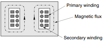
In most transformers there will be many turns on both windings, but for the sake of simplicity only four coils are shown for each winding. Operation of the transformer is explored in next article, but here we should recall that the purpose of a transformer is to take in electrical power at one voltage and supply it at a different voltage.
When an a.c. supply is connected to the primary winding, a pulsating magnetic flux (shown by the dotted lines in Figure 1) is set up. The pulsating flux links the secondary winding, inducing a voltage in each turn, so by choosing the number of turns in series the desired output voltage is obtained. Because no mechanical energy conversion is involved there is no need for an air-gap in the magnetic circuit, which therefore has an extremely low reluctance.
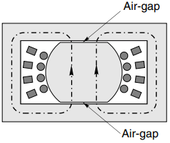
In Figure 1(b), we see a hypothetical set-up in which two small airgaps have been introduced into the magnetic circuit to allow for the motion that is essential in the induction motor.
Needless to say we would not do this deliberately in a transformer as it would cause an unnecessary increase in the reluctance of the flux path (though the effect on performance would be much less than we might fear). The central core and winding space have also been enlarged somewhat (anticipating the need for two more phases), without materially altering the functioning of the transformer.
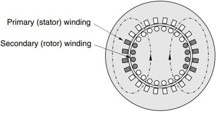
Finally, in Figure 1(c) we see the two sets of coils arranged as they would be in a 2-pole wound-rotor induction motor with full-pitched coils. The most important points to note are:
- Flux produced by the stator (primary) winding links the rotor (secondary) winding in much the same way as it did in Figure 1(a), i.e. the two windings remain tightly coupled by the magnetic field.
- Only one-third of the slots are taken up because the remaining two-thirds will be occupied by the windings of the other two phases: these have been omitted for the sake of clarity.
- The magnetic circuit has two air-gaps, and because of the slots that accommodate the coils, the flux threads its way down the teeth, so that it not only fully links the aligned winding, but also partially links the other two phase-windings.
- When the rotor turns, the rotor winding also turns and it therefore links less of the flux produced by the stator. If the rotor in Figure 1(c) turns through 90o, there will be no mutual flux linkage, i.e. the degree to which the two windings are magnetically coupled depends on the rotor position. If the two windings highlighted in Figure 1(c) were used as primary and secondary, this set-up would work perfectly well as a single-phase transformer.
We now turn to the theory of the transformer, to develop its equivalent circuit and in so doing lay the foundations for the induction motor equivalent circuit that is our ultimate objective.
Ideal Transformer & Real Transformer
To decrease the length of this webpage, content of these sections are published in next posts. To access those posts follow the links. Ideal Transformer and Real Transformer.
Development of Induction Motor Equivalent Circuit
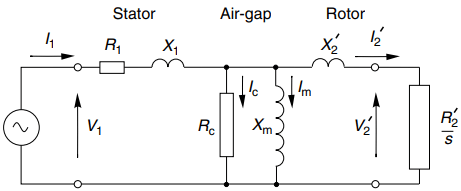
Stationary conditions: On a per-phase basis, the stationary induction motor is very much like a transformer, so to model the induction motor at rest we can use any of the transformer equivalent circuits we have looked at so far.
We can represent the motor at rest (the so-called ‘locked rotor’ condition) simply by setting Z2’ = 0 in ‘Approximate’ equivalent circuit of real transformer. (For a wound-rotor motor we would have to increase RT to account for any external rotor-circuit resistance.)
Given the applied voltage we can calculate the current and power that will be drawn from the supply, and if we know the effective turns ratio we can also calculate the rotor current and the power being supplied to the rotor.
But although our induction motor resembles a transformer, its purpose in life is very different because it is designed to convert electrical power to mechanical power, which of necessity involves movement.
Our locked-rotor calculations will therefore be of limited use unless we can calculate the starting torque developed. Far more importantly, we need to be able to represent the electromechanical processes that take place over the whole speed range, so that we can predict the input current, power and developed torque at any speed. The remarkably simple and effective way that this can be achieved is discussed next.
Modelling Electromechanical Energy Conversion Process
In previous articles, we saw that the behaviour of the motor was determined primarily by the slip. In particular we saw that if the motor was unloaded, it would settle at almost the synchronous speed (i.e. with a very small slip), with very little induced rotor current, at very low frequency.
As the load torque was increased the rotor slowed relative to the travelling flux; the magnitude and frequency of the induced rotor currents increased; the rotor thereby produced more torque; and the stator current and power drawn from the supply automatically increased to furnish the mechanical output power.
A very important observation in relation to what we are now seeking to do is that we recognised earlier that although the rotor currents were at slip frequency, their effect (i.e. their MMF) was always reflected back at the stator windings at the supply frequency.
This suggests that it must be possible to represent what takes place at slip-frequency on the rotor by referring the action to the primary (fixed-frequency) side, using a transformer-type model; and it turns out that we can indeed model the entire energy-conversion process in a very simple way.
All that is required is to replace the referred rotor resistance (R2’) with a fictitious slip-dependent resistance (R2’ = s) in the short-circuited secondary of our transformer equivalent circuit.
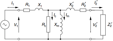
Hence if we build from the exact transformer circuit in Figure 2, we obtain the induction motor equivalent circuit shown in Figure 3. At any given slip, the power delivered to this ‘load’ resistance represents the power crossing the air-gap from rotor to stator.
We can see straightaway that because the fictitious load resistance is inversely proportional to slip, it reduces as the slip increases, thereby causing the power across the air-gap to increase and resulting in more current and power being drawn in from the supply.
This behaviour is of course in line with what we already know about the induction motor. There are two points worth making.
Firstly, given the complexity of the spatial and temporal interactions in the induction motor it is extraordinary that everything can be properly represented by such a simple equivalent circuit, and it has always seemed a pity to the author that something so elegant receives little by way of commendation in the majority of textbooks.
Secondly, the following brief discussion is offered for the benefit of readers who are seeking at least some justification for introducing the fictitious resistance R2’ = s, though it has to be admitted that full treatment is beyond our scope.
Pragmatists who are content to accept that the method works can jump to the next section. The key to developing the representation lies in ensuring that the magnitude and phase of the referred rotor current (at supply frequency) in the transformer model is in agreement with the actual current (at slip frequency) in the rotor.
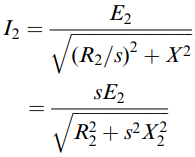
The induced e.m.f. in the rotor at slip s would be sE2 at frequency sf, where E2 is the e.m.f. induced under locked rotor (s = 1) conditions, when the rotor frequency is the same as the supply frequency, i.e. f.
This e.m.f. acts on the series combination of the rotor resistance R2 and the rotor leakage reactance, which at frequency sf is given by sX2, where X2 is the rotor leakage reactance at supply frequency. Hence the magnitude of the rotor current is given by
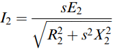
In the supply-frequency equivalent circuit, the secondary e.m.f. is E2, rather than sE2, so to obtain the same current in this model as given by equation (1), we require the slip-frequency rotor resistance and reactance to be divided by s, in which case the secondary current would be correctly given by
Properties of Induction Motors
We have started with the exact circuit in Figure 3 because the air-gap in the induction motor causes its magnetising reactance to be lower than a transformer of similar rating, while its leakage reactance will be higher. We therefore have to be a bit more cautious before we make major simplifications, though we will find later that for many purposes the approximate circuit (with the magnetising branch on the left) is actually adequate.
In this section, we concentrate on what can be learned from a study of the rotor section, which is the same in exact and approximate circuits, so our conclusions from this section are completely general.
Of the power that is fed across the air-gap into the rotor, some is lost as heat in the rotor resistance, and the remainder (hopefully the majority!) is converted to useful mechanical output power.
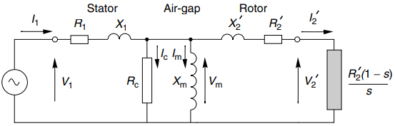
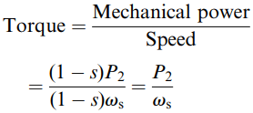
To represent this in the referred circuit we split the fictitious resistance R2’/s into two parts, R2’ and R2’((1-s)/s), as shown in Figure 4. The rotor copper loss is represented by the power in R2’, and the useful mechanical output power is represented by the power in the ‘electromechanical’ resistance R2’((1-s)/s), shown shaded in Figure 4.
To further emphasise the intended function of the motor – the production of mechanical power – the electromechanical element is shown in Figure 4 as the secondary ‘load’ would be in a transformer.
For the motor to be a good electromechanical energy converter, most of the power entering the circuit on the left must appear in the electromechanical load resistance. This is equivalent to saying that for good performance, the output voltage V2’ must be as near as possible to the input voltage, V1.
And if we ignore the current in the centre magnetising branch, the ‘good’ condition simply requires that the load resistance is large compared with the other series elements. This desirable condition is met under normal running condition, when the slip is small and hence R2’((1-s)/s) is large.
Our next step is to establish some important general formulae, and draw some broad conclusions.
Power balance: The power balance for the rotor can be derived as follows:
Power into rotor (P2) = Power lost as heat in rotor conductors + Mechanical output power.
Hence using the notation in Figure 4 we obtain
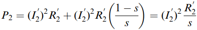
We can rearrange equation (3) to express the power loss and the mechanical output power in terms of the air-gap power, P2 to yield
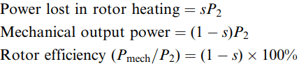
These relationships are of fundamental importance and universal applicability. They show that of the power delivered across the air-gap fraction s is inevitably lost as heat, leaving the fraction (1 – s) as useful mechanical output. Hence an induction motor can only operate efficiently at low values of slip.
Torque: We can also obtain the relationship between the power entering the rotor and the torque developed. We know that mechanical power is torque times speed, and that when the slip is s the speed is (1 – s)ωs, where ωs is the synchronous speed. Hence from the power equations above we obtain
Again this is of fundamental importance, showing that the torque developed is proportional to the power entering the rotor. All of the relationships derived in this section are universally applicable and do not involve any approximations.
Further useful deductions can be made when we simplify the equivalent circuit.
Approximate Equivalent Circuit of Induction Motor
This section is devoted to what can be learned from the equivalent circuit in simplified form, beginning with the circuit shown in Figure 5, in which the magnetising branch has been moved to the left-hand side. This makes calculations very much easier because the current and power in the magnetising branch are independent of the load branch.
The approximation involved in doing this are greater than in the case of a transformer because for a motor the ratio of magnetising reactance to leakage reactance is lower, but algebraic analysis is much simpler and the results can be illuminating.
A cursory examination of electrical machines textbooks reveals a wide variety in the approaches taken to squeeze value from the study of the approximate equivalent circuit, but in the author’s view there are often so many formulae that the reader becomes overwhelmed. So here we will focus on two simple messages.
Firstly, we will develop an expression that neatly encapsulates the fundamental behaviour of the induction motor, and illustrates the trade-offs involved in design; and secondly we will examine how the relative values of rotor resistance and reactance influence the shape of the torque–speed curve.
Starting and Full-Load Relationships
Straightforward circuit analysis of the circuit in Figure 5, together with equation (4) for the torque yields the following expressions for the load component of current (I2’) and for the torque per phase:
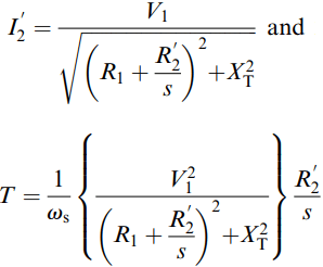
The second expression (with the square of voltage in the numerator) reminds us of the sensitivity of torque to voltage variation, in that a 5% reduction in voltage gives a little over 10% reduction in torque.
If we substitute s = 1 and s = sfl in these equations we obtain expressions for the starting current, the full-load current, the starting torque and the full-load torque.
Each of these quantities is important in its own right, and they all depend on the rotor resistance and reactance. But by combining the four expressions we obtain the very far-reaching result given by equation (7) below.
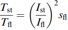
The left-hand side of equation (7) is the ratio of starting torque to full-load torque, an important parameter for any application as it is clearly no good having a motor that can drive a load once up to speed, but either has insufficient torque to start the load from rest, or (perhaps less likely) more starting torque than is necessary leading to a too rapid acceleration.
On the right-hand side of equation (7), the importance of the ratio of starting to full-load current has already been emphasised: in general it is desirable to minimise this ratio in order to prevent voltage regulation at the supply terminals during a direct-on-line start.
The other term is the full-load slip, which, as we have already seen should always be as low as possible in order to maximise the efficiency of the motor.
The remarkable thing about equation (7) is that it neither contains the rotor or stator resistances, nor the leakage reactances. This underlines the fact that this result, like those given in equations (4) and (5), reflects fundamental properties that are applicable to any induction motor. The inescapable design trade-off faced by the designer of a constant-frequency machine is revealed by equation (7).
We usually want to keep the full-load slip as small as possible (to maximise efficiency), and for direct starting the smaller the starting current, the better. But if both terms on the right-hand side are small, we will be left with a low starting torque, which is generally not desirable, and we must therefore seek a compromise between the starting and full-load performances.
It has to be acknowledged that the current ratio in equation (7) relates the load (rotor branch) currents, the magnetising current having been ignored, so there is inevitably a degree of approximation. But for the majority of machines (i.e. 2-pole and 4-pole) equation (7) holds good, and in view of its simplicity and value it is surprising that it does not figure in many ‘machines’ textbooks.
Dependence of Pull Out Torque on Motor Parameters
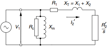
The aim here is to quantify the dependence of the maximum or pull-out torque on the rotor parameters, for which we make use of the simplest possible (but still very useful) model shown in Figure 6. The magnetising branch and the stator resistance are both ignored, so that there is only one current, the referred rotor current I2’ being the same as the stator current I1. Of the two forms shown in Figure 6, we will focus on the one in Figure 6(b), in which the actual and fictitious rotor resistances are combined.
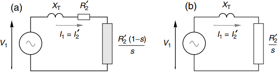
Most of the discussion will be based on normal operation, i.e. with a constant applied voltage at a constant frequency. In practice both leakage reactance and rotor resistance are parameters that the designer can control, but to simplify matters here we will treat the reactance as constant and regard the rotor resistance as a variable.
We will derive the algebraic relations first, then turn to a more illuminating graphical approach. To obtain the torque–slip relationship we will make use of equation (4), which shows that the torque is directly proportional to the total rotor power.
Throughout this section our main concern will be with how motor behaviour depends on the slip, particularly over the motoring region from s = 0 to s = 1. (The treatment can easily be extended to cover the braking and generating regions, but they are not included here.)
Analysis
The total rotor power per phase is given by
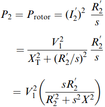
The bracketed expression on the right-hand side of equation (8) indicates how the torque varies with slip.
At low values of slip (i.e. in the normal range of continuous operation) where sX is much less than the rotor resistance R2’, the torque becomes proportional to the slip and inversely proportional to the rotor resistance. This explains why the torque–speed curves are linear in the normal operating region, and why the curves become steeper as the rotor resistance is reduced.
At the other extreme, when the slip is 1 (i.e. at standstill), we usually find that the reactance is larger than the resistance, in which case the bracketed term in equation (8) reduces to R2’/X2. The starting torque is then proportional to the rotor resistance.
By differentiating the bracketed expression in equation (8) with respect to the slip, and equating the result to zero, we can find the slip at which the maximum torque occurs. The slip for maximum torque turns out to be given by
s = R2’/XT ………(equation 9)
(A circuit theorist could have written down this expression by inspection of Figure 6, provided that he knew that the condition for maximum torque was that the power in the rotor was at its peak.)
Substituting the slip for maximum torque in equation (8), and using equation (5) we obtain an expression for the maximum torque per phase as:
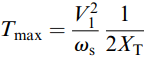
From these two equations we see that the slip at which maximum torque is developed is directly proportional to the rotor resistance, but that the peak torque itself is independent of the rotor resistance, and depends inversely on the leakage reactance.
Measurement of Parameters
The tests used to obtain the equivalent circuit parameters of a cage induction motor are essentially the same as those described for the transformer. To simulate the ‘open-circuit’ test we would need to run the motor with a slip of zero, so that the secondary (rotor) referred resistance (R2’/s) became infinite and the rotor current was absolutely zero.
But because the motor torque is zero at synchronous speed, the only way we could achieve zero slip would be to drive the rotor from another source, e.g. a synchronous motor. This is hardly ever necessary because when the shaft is unloaded the no-load torque is usually very small and the slip is sufficiently close to zero that the difference does not matter.
From readings of input voltage, current and power (per phase) the parameters of the magnetising branch (see Figure 5) are derived as described earlier. The no-load friction and windage losses will be combined with the iron losses and represented in the parallel resistor – a satisfactory practice as long as the voltage and/or frequency remain constant.
The short-circuit test of the transformer becomes the locked-rotor test for the induction motor. By clamping the rotor so that the speed is zero and the slip is one, the equivalent circuit becomes the same as the short-circuited transformer. The total resistance and leakage reactance parameters are derived from voltage, current and power measurements as already described.
With a cage motor the rotor resistance clearly cannot be measured directly, but the stator resistance can be obtained from a d.c. test and hence the referred rotor resistance can be obtained.