Equivalent Circuit of Real Transformer
We turn now to the real transformer, with the aim of developing its equivalent circuit. Real transformers behave much like ideal ones (except in very small sizes), and the approach is therefore to extend the model of the real transformer to allow for the imperfections of the real one.
For the sake of completeness we will establish the so-called ‘exact’ equivalent circuit first on a step-by-step basis. As its name implies the exact circuit can be used to predict all aspects of transformer performance, but we will find that it looks rather fearsome, and is not well adapted to offering simple insights into transformer behaviour.
Fortunately, given that we are not seeking great accuracy, we can retreat from the complexity of the exact circuit and settle instead for the much less daunting ‘approximate’ circuit which is more than adequate for yielding answers to the questions we need to pursue, not only for the transformer itself but also when we model the induction motor.
Real Transformer – No Load Condition
In modelling the real transformer at no-load we take account of the finite resistances of the primary and secondary windings; the finite reluctance of the magnetic circuit; and the losses due to the pulsating flux in the iron core.
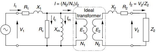
The winding resistances are included by adding resistances R1 and R2, respectively in series with the primary and secondary of the ideal transformer, as shown in Figure 1.
The transformer in Figure 1 is shown without a secondary load i.e. it is under no-load conditions. As previously explained the current drawn from the supply in this condition is known as the magnetising current, and is therefore denoted by Im.
Because the ideal transformer (within the dotted line in Figure 1) is on open-circuit, the secondary current is zero and so the primary current must also be zero.
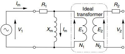
So to allow for the fact that the real transformer has a no-load magnetising current we add an inductive branch (known as the ‘magnetising reactance’) in parallel with the primary of the ideal transformer, as shown in Figure 1.
In circuit theory terms, the magnetising reactance is simply the reactance due to the self-inductance of the primary of the transformer. Its value reflects the magnetising current, as discussed later.
We now need to recall that when we apply Kirchoff’s law to the primary winding, we obtain equation
V1 = E1 + ImR1 …….(equation 1)
Which includes the term ImR1, the volt-drop across the primary resistance due to the magnetising current.
It turns out that when a transformer is operated at its rated voltage, the term ImR1 is very much less than V1, so we can make the approximation V1∼E1, i.e. in a real transformer the induced e.m.f. is equal to the applied voltage, just as in the ideal transformer.
This is a welcome news as it allows us to use the simple design equation linking flux, voltage and turns (developed in previous article for the ideal transformer) for the case of the real transformer.
More importantly, we can continue to say that the flux will be determined by the applied voltage, and it will not depend on the reluctance of the magnetic circuit. However, the magnetic circuit of the real transformer clearly has some reluctance, so it is to be expected that it will require a current to provide the MMF needed to set up the flux in the core.
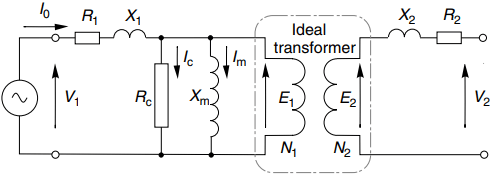
If the reluctance is R and the peak flux is ɸm, the magnetic Ohm’s law gives
The magnetising reactance Xm is given by Xm = V1 / Im ……..(equation 3)
In most transformers the reluctance of the core is small, and as a result the magnetising current (Im) is much smaller than the normal full-load (rated) primary current. The magnetising reactance is therefore high, and we will see that it can be neglected for many purposes.
However, the induction motor (our ultimate goal!) resembles a transformer with two air-gaps in its magnetic circuit. If we were to simulate the motor magnetic circuit by making a couple of saw-cuts across our transformer core, the reluctance of the magnetic circuit would clearly be increased because, relative to iron, air is a very poor magnetic medium.
Indeed, unless the saw-blade was exceptionally thin we would probably find that the reluctance of the two air-gaps greatly exceeded the reluctance of the iron core. We might have thought that making saw-cuts and thereby substantially increasing the reluctance would reduce the flux in the core, but we need to recall that provided the term ImR1 is very much less than V1, the flux is determined by the applied voltage, and the magnetising current adjusts to suit, as given by equation (2).
So when we make the sawcuts and greatly increase the reluctance, there is a compensating large increase in the magnetising current, but the flux remains virtually the same. We can see that there must be a small reduction in the flux when we increase the reluctance by rearranging equation (1) in the form:
Im = (V1 – E1)/R1
From which we can see that the only way that Im can increase to compensate for an increase in the reluctance is for E1 to reduce. However, since E1 is very nearly equal to V1, a very slight reduction in E1 (and hence a very slight reduction in flux) is sufficient to yield the required large increase in the magnetising current.
The final refinement of the no-load model takes account of the fact that the pulsating flux induces eddy current and hysteresis losses in the core. The core is laminated to reduce the eddy current losses, but the total loss is often significant in relation to overall efficiency and cooling, and we need to allow for it in our model.
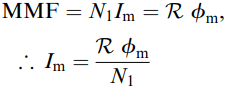
The iron losses depend on the square of the peak flux density, and they are therefore proportional to the square of the induced e.m.f. This means that we can model the losses simply by including a resistance (Rc – where the suffix denotes ‘core loss’) in parallel with the magnetising reactance, as shown in Figure 2.
The no-load current (I0) consists of the reactive magnetising component (Im) lagging the applied voltage by 90o, and the core-loss (power) component (Ic) that is in phase with the applied voltage.
The magnetising component is usually much greater than the core-loss component, so the real transformer looks predominantly reactive under open-circuit (no-load) conditions.
Real Transformer – Leakage Reactance
In the ideal transformer it was assumed that all the flux produced by the primary winding linked the secondary, but in practice some of the primary flux will exist outside the core and will not link with the secondary.
This leakage flux, which is proportional to the primary current, will induce a voltage in the primary winding whenever the primary current changes, and it can therefore be represented by a ‘primary leakage inductance’ (l1) in series with the primary winding of the ideal transformer.
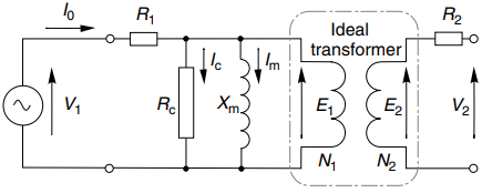
We will normally be using the equivalent circuit under steady-state operating conditions at a given frequency (f), in which case we are more likely to refer to the ‘primary leakage reactance’ (X1 = ωl1 = 2πfl1) as in Figure 3.
The induced e.m.f. in the secondary winding arising from the secondary leakage flux (and thus proportional to the secondary current) is modeled in a similar way, and this is represented by the ‘secondary leakage reactance’ (X2) shown in Figure 3.
It is important to point out that under no-load conditions when the primary current is small the volt-drop across X1 will be much less than V1, so all our previous arguments relating to the relationship between flux, turns and frequency can be used in the design of the real transformer.
Because the leakage reactances are in series, their presence is felt when the currents are high, i.e. under normal full-load conditions, when the volt-drops across X1 and X2 may not be negligible, and especially under extreme conditions (e.g. when the secondary is short-circuited) when they provide a vitally important current-limiting function.
Looking at Figure 3 the conscientious reader could be forgiven for beginning to feel a bit downhearted to discover how complex matters appear to be getting, so it will come as good news to learn that we have reached the turning point.
The circuit in Figure 3 represents all aspects of transformer behaviour if necessary, but it is more elaborate than we need, so from now on things become simpler, particularly when we take the usual step and refer all secondary parameters to the primary.
Real Transformer on Load – Exact Equivalent Circuit
The equivalent circuit showing the transformer supplying a secondary load impedance Z2 is shown in Figure 4(a). This diagram has been annotated to show how the ideal transformer at the centre imposes the relationships between primary and secondary currents.
Provided that we know the values of the transformer parameters we can use this circuit to calculate all the voltages, currents and powers when either the primary or secondary voltage are specified. However, we seldom use the circuit in this form, as it is usually much more convenient to work with the referred impedances.
From the primary viewpoint, we can model the combination of ideal transformer and its load by ‘referring’ the secondary impedance to the primary. Also, an impedance Z2 connected to the secondary can be modelled by a referred impedance Z’2 connected at the primary, where Z’2 = (N1/N2)2 ÷ Z2.
We can use the same approach to refer not only the secondary load impedance Z2 but also the secondary resistance and leakage reactance of the transformer itself, as shown in Figure 4(b).
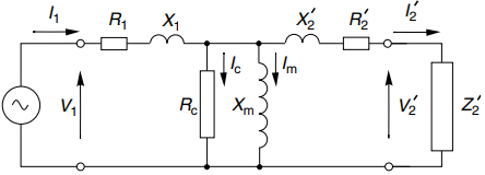
As before, the referred or effective load impedance, secondary resistance and leakage reactance as seen at the primary are denoted by Z’2, R’2 and X’2, respectively.
When circuit calculations have been done using this circuit the actual secondary voltage and current are obtained from their referred counterparts using the equations
V2 = V’2(N2/N1) and
I2 = I’2(N1/N2) …………(equation 4)
At this point we should recall the corresponding circuit of the ideal transformer. There we saw that the referred secondary voltage V’2 was equal to the primary voltage V1.
For the real transformer, however, (Figure 4(b)) we see that the imperfections of the transformer are reflected in circuit elements lying between the input voltage V1 and the secondary voltage V’2, i.e. between the input and output terminals.
In the ideal transformer the series elements (resistances and leakage reactances) are zero, while the parallel elements (magnetising reactance and core-loss resistance) are infinite.
The principal effect of the non-zero series elements of the real transformer is that because of the volt-drops across them, the secondary voltage V’2 will be less than it would be if the transformer were ideal. And the principal effect of the parallel elements is that the real transformer draws a (magnetising) current and consumes (a little) power even when the secondary is open-circuited.
Although the circuit of Figure 4(b) represents a welcome simplification compared with that in Figure 4(a), calculations are still cumbersome, because for a given primary voltage, every volt-drop and current changes whenever the load on the secondary alters.
Fortunately, for most practical purposes a further gain in terms of simplicity (at the expense of only a little loss of accuracy) is obtained by simplifying the ‘exact’ circuits in Figure 4 to obtain the so-called ‘approximate’ equivalent circuit.
Real Transformer – Approximate Equivalent Circuit
The justification for the approximate equivalent circuit (see Figure 5(a)) rests on the fact that for all transformers except very small ones the series elements in Figure 4(b) are of low impedance and the parallel elements are of high impedance. Actually, to talk of low or high impedances without qualification is nonsense.
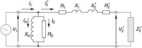
What the rather loose language in the paragraph above really means is that under normal conditions, the volt-drop across R1 and X1 will be a small fraction of the applied voltage V1.
Hence the voltage across the magnetising branch (Xm in parallel with Rc) is almost equal to V1: so by moving the magnetising branch to the left-hand side, the magnetising current and the core-loss current will be almost unchanged. Moving the magnetising branch brings massive simplification in terms of circuit calculations.
Firstly because the current and power in the magnetising branch are independent of the load current, and secondly because primary and referred secondary impedances now carry the same current (I’2) so it is easy to calculate V’2 from V1 or vice-versa.
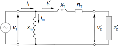
Further simplification results if we ignore the resistance (Rc) that models iron losses in the magnetic circuit, and we combine the primary and secondary resistances and leakage reactances to yield total resistance (RT) and total leakage reactance (XT) as shown in Figure 5(b).
The justification for ignoring the iron-loss resistance is that the eddy current and hysteresis losses in the iron are only of interest when we are calculating efficiency, which is not our concern here, and in most transformers the associated current (Ic) is small, so ignoring it has little impact on the total input current.
Given the difference in the numbers of turns and wire thickness between primary and secondary windings it is not surprising that the actual primary and secondary resistances are sometimes very different.
But when referred to the primary, the secondary resistance is normally of similar value to the primary resistance, so both primary and secondary contribute equally to the total effective resistance.
This is in line with commonsense: since both windings contain the same quantities of copper and handle the same power, both would be expected to have similar influence on the overall performance.
When leakage reactances are quoted separately for primary and secondary they too may have very different ohmic values, but again when the secondary is referred its value will normally be the same as that of the primary.
In fact, the validity of regarding leakage reactance as something that can be uniquely apportioned between primary and secondary is questionable, as they cannot be measured separately, and for most purposes all that we need to know is the total leakage reactance XT.
The equivalent circuit in Figure 5(b) will serve us well when we extend the treatment to the induction motor. It is delightfully simple, having only three parameters, i.e. the magnetising reactance Xm, the total leakage reactance XT and the total effective resistance RT.
Measurement of Parameters
Two simple tests are used to measure the transformer parameters – the open-circuit or no-load test and the short-circuit test. We will see later that very similar tests are used to measure induction motor parameters.
In the open-circuit test, the secondary is left disconnected and with rated voltage (V1) applied to the primary winding, the input current (I0) and power (W0) are measured. If we are seeking values for the three-element model in Figure 5(b), we would expect no power at no load, because the only circuit is that via the magnetising reactance Xm.
So if, as is usually the case, the no-load input power W0 is very much less than V1I0 (i.e. the transformer looks predominantly reactive) we assume that the input current I0 is entirely magnetising current and deduce the value of the magnetising reactance from
Xm = V1/I0
(If we want to use the more accurate model in Figure 5(a), we note that the input power will be solely that due to the iron loss in the resistor Rc.
Hence W0 = V12 /Rc, i.e. Rc = V12/W0.)
In the short-circuit test the secondary terminals are shorted together and a low voltage is applied to the primary – just sufficient to cause rated current in both windings. The voltage (Vsc), current (Isc) and input power (Wsc) are measured.
In this test, Xm is in parallel with the impedance ZT (i.e. the series combination of XT and RT), so the input current divides between the two paths. However, the reactance Xm is invariably very much larger than the impedance ZT, so we usually neglect the small current through Xm and assume that the current Isc flows only through ZT. The resistance can then be derived from the input power using the relationship:
Wsc = I2sc RT, ; RT = Wsc /I2sc
And the leakage reactance can be derived from
ZT = Vsc /Isc = √(RT2 + XT2)
To split the resistances, the primary and/or secondary winding resistances are measured under d.c. conditions.
A great advantage of the open-circuit and short-circuit tests is that neither require more than a few per cent of the rated power, so both can be performed from a modestly rated supply.
Significance of Equivalent Circuit Parameters
If the study of transformers was our aim, we would now turn to some numerical examples to show how the equivalent circuit was used to predict performance: for example, we might want to know how much the secondary voltage dropped when we applied the load, or what the efficiency was at various loads.
But our aim is to develop an equivalent circuit to illuminate induction motor behaviour, not to become experts at transformer analysis, so we will avoid quantitative study at this point.
On the other hand, as we will see, the similarities with the induction motor circuit mean that there are several qualitative observations that are worth making at this point.
Firstly, if it were possible to choose whatever values we wished for the parameters, we would probably look back at the equivalent circuit of the ideal transformer, and try to emulate it by making the parallel elements infinite, and the series elements zero.
And if we only had to think about normal operation (from no-load up to rated load) this would be a sensible aim, as there would then be no magnetising current, no iron losses, no copper losses and no drop in secondary voltage when the load is applied.
Most transformers do come close to this ideal when viewed from an external perspective. At full load the input power is only slightly greater than the output power (because the losses in the resistive elements are a small fraction of the rated power); and the secondary voltage falls only slightly from no-load to full-load conditions (because the volt-drop across ZT at full-load is only a small fraction of the input voltage).
But in practice we have to cope with the abnormal as well as the normal, and in particular we need to be aware of the risk of a short-circuit at the secondary terminals.
If the transformer primary is supplied from a constant-voltage source, the only thing that limits the secondary current if the secondary is inadvertently short-circuited is the series impedance ZT. But we have already seen that the volt-drop across ZT at rated current is only a small fraction of the rated voltage, which means that if rated voltage is applied across ZT, the current will be many times a rated value. So the lower the impedance of the transformer, the higher the short-circuit current.
From the transformer viewpoint, a current of many times rated value will soon cause the windings to melt, to say nothing of the damaging inter-turn electromagnetic forces produced. And from the supply viewpoint the fault current must be cleared quickly to avoid damaging the supply cables, so a circuit breaker will be required with the ability to interrupt the short-circuit current.
The higher the fault current, the higher the cost of the protective equipment, so the supply authority will normally specify the maximum fault current that can be tolerated.
As a transformer designer we then face a dilemma: if we do what seems obvious and aim to reduce the series impedance to improve the steady-state performance, we find that the short-circuit current increases and there is the problem of exceeding the permissible levels dictated by the supply authority.
Clearly the so-called ideal transformer is not what we want after all, and we are obliged to settle for a compromise. We deliberately engineer sufficient impedance (principally via the control of leakage reactance) to ensure that under abnormal (short-circuit) conditions the system does not self-destruct!
This is very similar in relation to the induction motor: when the induction motor is started direct-on-line it draws a heavy current, and limiting the current requires compromises in the motor design. We will see shortly that this behaviour is exactly like that of a short-circuited transformer.