This article focuses on a motor intended for motion control—the servomotor, or servo. Whereas stepper motors rotate through an angle and halt, many servo motors rotate continuously. Properly controlled, a servo can do everything a stepper can and more.

In addition to setting the rotation angle, the controller can configure the servo’s rotational speed and acceleration. This added control is the main advantage of servos over steppers. The main disadvantage is that designing a servo controller is a difficult process.

A stepper can be controlled with a simple sequence of discrete pulses. With servos, the control signals are more involved. The goal of this article is to explain why this is the case and to show how this control can be accomplished. It’s important to note that the term servomotor doesn’t imply anything about the motor’s structure.

A servo may be brushed or brushless, AC or DC. The fundamental difference between servomotors and other electric motors is the availability of position feedback.

A servo sends a signal to the controller that identifies its rotation angle and/or rotation speed. The controller uses this feedback to determine what control signals to send.

Unfortunately, most servos directed toward hobbyists don’t provide feedback. I’ll refer to these as hobbyist servos, and the first part of this article presents them in detail.

We’ll also look at encoders, which are systems that can be connected to motors to provide feedback. The rest of the article focuses on servos that deliver feedback to the controller. Designing a controller for this kind of servo requires mathematical modeling—a model of the servo and a model of the controller’s signals.

The benefit of this modeling is that the motor can be made to turn with incredible precision. The drawback is that the mathematical theory has a significant learning curve.

Hobbyist Servo Motor

Judging from the websites that cater to hobbyists, the main vendors that make hobbyist servos are Hitec, Fitec, Futaba, and Tower Pro. It’s possible that one of their offerings provides position feedback, but I’ve never encountered any. Most hobbyist servos have a boxlike shape with three wires. Figure 1 shows what the FS5106B servo from Fitec (frequently spelled FeeTech) looks like.

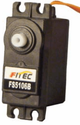
The three wires connect the motor to power, ground, and the controller. Additional information can be obtained from its datasheet:

• Internal structure: Brushed DC motor
• Input voltage: 4.8 – 6 V
• Stall torque: 69.56 oz-in. (4.8 V) or 83.47 oz-in. (6.0 V)
• No-load speed: 55.5 RPM (4.8 V) or 62.5 RPM (6.0 V)
• Running degree: 180° ± 5°
• Pulse width range: 0.7 – 2.3 ms
• Neutral position: 1.5 ms
• Dead bandwidth: 0.005 ms

The first four parameters should be clear. The FS5106B servo is based on a brushed DC motor that accepts between 4.8 V and 6.0 V. The torque and speed depend on how much voltage is provided. The last four parameters may not be clear. They define the nature of the servo’s motion and the type of signals needed to control it. This section explores both topics.

PWM Control of Servo Motor

DC motors can be controlled by sending pulse width modulation (PWM) signals. The PWM delivers pulses of varying width to the motor. Figure 2 provides a simple example.

As given by the “running degree” parameter, the FS5106B’s rotor can turn 180°. The controller sets the rotor’s angle by sending pulses to the servo and controlling the width of each pulse.

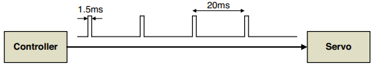
According to the “pulse width range” parameter, the servo responds to pulses whose widths are between 0.7 ms and 2.3 ms. The neutral position is set when the pulse width is at 1.5 ms, which is the pulse width illustrated in Figure 2 .

Similarly, a pulse width of 0.7 ms turns the rotor to the full left position, and a pulse width of 2.3 ms sets the rotor to the full right position. In theory, we’d like the servo to turn every time the pulse width changes.

But in practice, the servo should ignore minor deviations in pulse width that may have been caused by noise. This is the meaning of the “dead bandwidth” parameter, which equals 0.005 ms for the FS5106B. If the pulse width changes by less than 0.005 ms, the servo won’t move.

When power is turned off, the servo’s rotor stays in its position. This means that, when power is turned on again, the controller may not know the rotor’s angle. For this reason, it’s common to return the servo to the neutral position as soon as power becomes available.

The controllers govern a servo’s behavior with PWM. An Arduino circuit board can be programmed to control servomotors. A Raspberry Pi single-board computer can generate PWM pulses for servos.

Analog and Digital Servos

According to its specification, the FS5106B is an analog servo instead of a digital servo. From the controller’s perspective, there’s no difference between the two—both types are controlled by the same PWM signals. The difference involves the internal circuitry that receives control signals and delivers power to the motor.

When an analog servo receives pulses from the controller, it amplifies them and sends them to the motor to provide power. As the rotor approaches the desired position, the power diminishes to zero. If the widths of the incoming pulses are less than the servo’s dead bandwidth (0.005 ms in the case of the FS5106B), the motor won’t receive any power.

Digital servos operate in essentially the same way, but a digital servo has a microprocessor that receives pulses from the controller, processes them, and delivers pulses to the motor. The presence of the microprocessor provides three advantages:

• Lower dead bandwidth— The processor can respond to pulses that are too small for an analog servo to notice.
• Higher-frequency power— The pulses sent by the processor have a higher frequency than those sent by the controller. This makes digital servos more responsive than analog servos.
• Programmability— The processor’s operating characteristics can be configured by the user.

This last point is particularly interesting. Many vendors of digital servos provide programming tools capable of setting the operating parameters of their motors. For example, a digital servo from Hitec can be programmed with Hitec’s HFP-10 programmer, which can set the following parameters:

• Direction— Clockwise or counterclockwise
• Speed— Rotation speed in RPM
• Left endpoint/right endpoint— Maximum angles that can be reached
• Dead bandwidth— Minimum pulse width (in microseconds) that the servo will respond to
• Failsafe— The servo’s behavior when the connection to the controller is cut off

There are two significant disadvantages of using digital servos. The first is cost. Digital servos generally cost twice as much as comparable analog servos. The second disadvantage involves power. Because of its microprocessor, a digital servo requires more power than a comparable analog servo.

A minor disadvantage of digital servos relates to the dead bandwidth. By default, a digital servo responds to small changes in pulse width that an analog servo would ignore. This can be a problem in noisy environments, draining current from the power supply. However, if the servo’s dead bandwidth is suitably configured with a programmer, this won’t be an issue.

Rotary Encoders

To convert a hobbyist servo (or any electric motor) to a proper servomotor, a mechanism must be attached that identifies the shaft’s angle. These feedback elements are called rotary encoders. Many types of encoders are available, but for servo applications, there are two main choices:

• Optical— A sensor detects light passing through a specially patterned disk.
• Magnetic— A sensor detects the moving poles of a magnet. This discussion presents both types of encoders.

Optical Encoders: Of the many encoders used with servos, optical encoders are the simplest and most common. Their operation is made possible by a disk connected to the motor’s shaft. This disk is transparent in some areas and opaque in others.

On one side of the disk, a light source directs light at one portion of the disk. On the other side, an optical sensor measures how much light passes through. The sensor delivers its results to a processor, which may assign a 1 to the presence of light and a 0 to the absence. The disk’s pattern of transparent and opaque regions usually takes one of two forms. Figure 3 illustrates both patterns.

The disk on the left has alternating stripes of transparent and opaque regions. As the shaft turns, the optical sensor measures the time between successive flashes of light. The processor uses this to determine how quickly the motor’s shaft is turning. Because it provides speed but not position, this type of encoder is called an incremental encoder .

In contrast, the disk on the right of Figure 3 is used by absolute encoders because it identifies the shaft’s angle as well as its speed. In this case, the light shines along an axial stripe that has alternating transparent/opaque regions.

The optical sensor detects this light and passes multiple readings to the processor. The microprocessor converts the pattern of light and darkness into a number and uses it to determine the shaft’s approximate angle.

Magnetic Encoders: Optical encoders are more common, but magnetic encoders are generally more reliable and provide better resolution. In these encoders, a circular magnet is attached to the shaft. A magnetic sensor is positioned close to the magnet to detect its north and south poles. As the shaft turns, the sensor measures the locations of the changing poles and determines the shaft’s angle and speed.

Overview of Servo Control

Stepper motors are very simple – a stepper’s shaft rotates through a specific angle and stops. But if you measure the shaft’s angle as it changes from the initial angle, θ_i , to the final angle, θ_f , you might see something like the graph in Figure 4 As shown, the shaft needs time to ramp up and its angle oscillates before reaching its final angle.

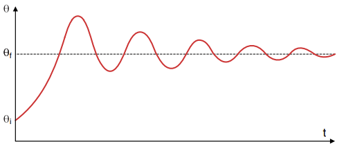
Hobbyist servos behave in the same manner. If the motor is intended for a radio-controlled aircraft or a paper printer, this isn’t a significant concern. However, if the intended application requires high-precision motor control, such in the case of robotic surgery, you shouldn’t insert a stepper motor and hope for the best.

You need a precise understanding of how the motor behaves when it receives signals from the controller. In addition, if the load changes over time, the controller needs to know how to maintain the rotor’s motion.

The goal of control theory is to make this fine-tuned control possible. To accomplish this goal, it uses mathematical representations of the motor and the controller’s signals.

Open-Loop and Closed-Loop Systems

If a controller receives feedback identifying a servo’s shaft angle, it can measure the angle over time to determine the motor’s speed and acceleration. If the motor deviates from the desired behavior, the controller will send control signals to reduce the deviation.

This exchange of information—the servo provides its position, the controller provides control signals—forms a loop. For this reason, systems with feedback are referred to as closed-loop systems.

Systems without feedback are open-loop systems. The block diagrams in Figure 5 illustrate the difference between these two systems.

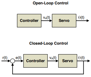
To analyze closed-loop systems mathematically, we represent each of the signals with functions that change over time. Here are the four functions commonly encountered in servomotor control:

• θ(t)— The angle of the servomotor’s shaft
• r(t)— The desired angle of the servomotor (called the reference or the setpoint )
• e(t)— The deviation (error) between the motor’s angle and the desired angle
• va(t)— The control signal (voltage) provided by the controller

For the purposes of this chapter, the controller’s signal, v_a(t), is an analog function of time. The primary question of servo control is how v_a(t) should be computed from e(t).

As a real-world example, consider a boat whose steering is automated by a computer. Using sonar, visual sensors, and weather databases, the computer determines what course to take. This set of angles forms the system’s setpoint, r(t). The controller receives r(t) and delivers a signal, v_a(t), to a servo connected to the ship’s rudder. As the servo turns, the rudder changes the boat’s heading, denoted as θ(t).

If wind blows the boat off-course, the error, e(t), equals the difference between r(t) and θ(t). The controller receives this error and adjusts v_a(t) to return to the boat to a suitable heading. This new v_a(t) is computed with the help of control theory.