Types of Oscilloscope
After the multimeter, the oscilloscope is the most commonly used item of electronic test equipment. Be it the electronics industry or a research laboratory, the oscilloscope is an indispensable test and measurement tool for an electronics engineer or technician.
Most of us regard the oscilloscope as an item of equipment that is used to see pulsed or repetitive waveforms. However, very few of us are familiar with the actual use of the multiplicity of front-panel controls on the oscilloscope and the potential that lies behind the operation of each one of these controls.
With the arrival of the digital storage oscilloscope (DSO), the functional potential of oscilloscopes has greatly increased. The digital storage oscilloscope enjoys a number of advantages over its analogue counterpart.
Types of Oscilloscope
Technology is often the single most important criterion forming the basis of oscilloscope classification. Different types of oscilloscope include analogue oscilloscopes, CRT storage type analogue oscilloscopes, digital storage oscilloscopes and sampling oscilloscopes.
Digital storage oscilloscopes and sampling oscilloscopes are often clubbed together under digital oscilloscopes. Analogue oscilloscopes are briefly described in the following paragraphs. This is followed up by a detailed description of digital oscilloscopes.
Analogue Oscilloscopes
The analogue oscilloscope displays the signal directly and enables us to see the waveform shape in real time. The signal update rate in an analogue oscilloscope is the fastest possible as there is only the beam retrace timing and the trigger rearm between two successive sweeps. Consequently, an analogue oscilloscope has a much higher probability of capturing the desired event than any other type of oscilloscope.
Analogue oscilloscopes find wide application for viewing both repetitive and single-shot events up to a bandwidth of about 500 MHz. Analogue oscilloscopes do not give a desirable display when viewing very low-frequency repetitive signals or single-shot events.
In such cases, the display is nothing but a bright dot moving slowly across the screen to trace the waveform. Such waveforms are not at all convenient to analyse and need some kind of photographic memory.
CRT Storage Type Analogue Oscilloscopes
A CRT storage type analogue oscilloscope overcomes this problem by using a special type of CRT. In one such type, the phosphor dots have higher persistence. As a result, the moving dot leaves behind a visible trail as it sweeps across the screen, even at much lower sweep speeds.
There are two main types of storage mode currently in use for these oscilloscopes: the bistable storage mode, which is capable of storing signals for many hours, and the more popular variable-persistence storage mode, which can store signals for a maximum of 10 min. The majority of commercially available CRT storage oscilloscopes have the option of both the above-mentioned storage modes.
The CRT storage type oscilloscope is an excellent choice for slowly changing signals. As the writing rate is faster than that of the conventional analogue oscilloscopes, it is extremely good for viewing fast transient events. It can be used to store both repetitive and single-shot signals having a bandwidth of up to 500 MHz or so.
Oscilloscope type 7934 from Tektronix, for instance, has a bandwidth of 500 MHz and a maximum writing speed of 4000 cm/ms. Even handheld versions of these scopes with a reasonably good writing speed are available.
Analogue storage oscilloscope technology is fast being replaced by digital storage oscilloscope technology owing to the far superior performance features of the latter.
Digital Oscilloscopes
In a digital oscilloscope, the signal to be viewed is firstly digitized inside the scope using a fast A/D converter. The digitized signal is stored in a high-speed semiconductor memory to be subsequently retrieved from the memory and displayed on the oscilloscope screen. There are two digitizing techniques, namely real-time sampling and equivalent-time sampling.
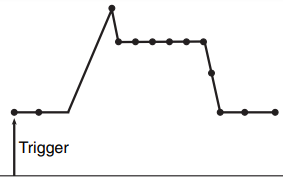
The digital storage oscilloscopes (DSOs) use real-time sampling, as shown in Fig. 1, so that they can capture both repetitive and single-shot signals. In digital storage oscilloscopes, the digitizer samples the entire input waveform with a single trigger. Sampling oscilloscopes use equivalent-time sampling and are limited to capturing repetitive signals.
Some digital storage oscilloscopes also use equivalent-time sampling to extend their useful frequency range for capturing repetitive signals. The equivalent-time sampling technique is thus applicable to only stable repetitive signals and can be implemented in at least three different ways, namely sequential single-sample, sequential sweep and random interleaved sampling (RIS).
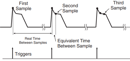
In the sequential single-sample technique (Fig. 2), the digitizer acquires a single sample with the first trigger pulse. It then waits for the second trigger, and, on receipt of the second trigger, a time delay equal to the reciprocal of the desired sampling rate is executed and then the second sample is acquired. The trigger-to-acquisition delay is incremented by the desired intersample period Δt for each subsequent acquisition. The resulting capture has thus an equivalent sample rate of 1/Δt.
Clearly, this method is slow, as N trigger cycles would be needed to gather N samples, and the scopes using this type of digitizing technique cannot provide real-time operation.
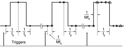
In sequential sweep equivalent-time sampling (Fig. 3), a sweep of samples spanning the desired display time range is acquired for each trigger. Here, N samples are acquired in M trigger cycles, where N = kM. On receipt of each trigger, k sequential samples are acquired at sample rate fs. These are stored in every Mth location of the acquisition memory allocated for N samples. k samples of the first sweep are acquired directly on receipt of the trigger.
Subsequent sweeps have an increasing delay between trigger receipt and sweep initiation, with the delay increment being equal to 1/Mfs with reference to trigger detection in order to give an apparent sample rate of Mfs.
The random interleaved sampling (RIS) technique uses a memory distribution scheme that is philosophically similar to that of sequential sweep equivalent-time sampling, with the difference that the samples are random with respect to the trigger. Sampling in this case occurs on both sides of trigger points, which gives this technique a ‘pretrigger view’ capability not available in the first two equivalent-time sampling techniques, as both methods gather signals only following the receipt of a trigger.
If we wanted to view a 1 GHz signal, the sweep speed requirement would be enormous. Even if we were successful in achieving this high speed, the beam would be almost invisible. We have often noticed that, as the time-base setting is made faster, we are forced to adjust the intensity control to maintain an acceptable intensity level setting.
Another major problem in designing a real-time oscilloscope for viewing very high-frequency signals (in the GHz range) is the difficulty in building such a high bandwidth in the vertical amplifier. A sampling oscilloscope using any of the equivalent-time sampling techniques outlined above is an answer to all these problems.
In such scopes it is not imperative to take a sample or a group of samples from each cycle of the signal to be viewed. The next adjacent sample or group of samples may be 10 000 cycles away. As a result, the bandwidth of the vertical amplifier can afford to be much lower than the frequency of the signal.
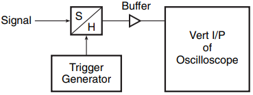
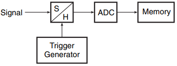
Another type of sampling oscilloscope, although not very common in use, is the analogue sampling oscilloscope, where a conventional sample/hold circuit consisting of an electronic switch and a capacitor is used for signal acquisition (Fig. 4). It can be used to view high-frequency repetitive signals in non-storage mode, unlike the digital sampling scopes where the signal is sampled digitally and then stored in semiconductor memory for subsequent retrieval.
It can also be used for viewing high-frequency repetitive signals in storage mode, although not in real time (Fig. 5). Digital storage oscilloscopes are also available in a large variety of sizes, shapes, performance features and specifications.
Battery-operated, handheld digital storage oscilloscopes with a bandwidth as high as 200 MHz are common. The digital phosphor oscilloscope (DPO) is a big step forward in DSO technology. It captures, stores, displays and analyses, in real time, three dimensions of signal information, i.e. amplitude, time and distribution of amplitude over time.
This third dimension offers the advantage of interpretation of signal dynamics, including instantaneous changes and the frequency of occurrence displayed in the form of quantitative intensity information.
Analogue versus Digital Oscilloscopes
Almost all oscilloscopes available today use one or a combination of the technologies discussed above. Each technology has its own benefits and shortcomings. While signal manipulation and its consequent benefits are the strong point of the digital technology, extremely fast update rates coupled with low cost is a feature associated with analogue scopes. In fact, many state-of-the-art oscilloscopes are not simply analogue or digital. They offer advantages of both technologies.
Oscilloscope Specifications
Although oscilloscopes are characterized by scores of performance specifications, not all of them are important. Important specifications of analogue and digital oscilloscopes are briefly described in the following paragraphs.
Analogue Oscilloscopes Key Specifications
Analogue Oscilloscopes Key specifications include bandwidth (or rise time), vertical sensitivity and accuracy. Other features such as triggering capabilities, display modes, sweep speeds, etc., are secondary in nature.
Bandwidth and Rise Time: The bandwidth and rise time specifications of an oscilloscope are related to one another. Each can be calculated from the other. Bandwidth (in MHz) = 350/rise time (in ns). Bandwidth is the most important specification of any oscilloscope. It gives us a fairly good indication of the signal frequency range that can be viewed on the oscilloscope with an acceptable accuracy.
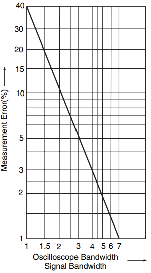
If we try to view a signal with a bandwidth equal to the bandwidth of the oscilloscope, the measurement error may be as large as 40 % (Fig. 7). As a rule, the oscilloscope bandwidth should be 3–5 times the highest frequency one is likely to encounter in order to keep the measurement error to less than 5 %.
Vertical sensitivity: The vertical sensitivity specification tells us about the minimum signal amplitude that can fill the oscilloscope screen in the vertical direction. A 5 mV/div sensitivity is quite common. Oscilloscopes with a sensitivity specification of 1 mV/div are also available.
Sensitivity and bandwidth are often trade-offs. Although a higher bandwidth enables us to capture high-frequency signals, there is a good possibility of unwanted high-frequency noise being captured if the oscilloscope has a higher sensitivity too.
That is why most of the high-sensitivity scopes have bandwidth limit controls to enable a clear view of low-level signals of moderate frequencies.
It is also important that the oscilloscope we choose has an adequate V/div range to make possible a full-screen or near-full-screen display for a wide range of signal amplitudes.
Accuracy: The accuracy specification indicates the degree to which our measurement conforms to a true and accepted standard value. An accuracy of ±1 − 3% is typical. Almost all oscilloscopes are provided with a ×5 magnification in the V/div selector switch. This alters the nominal vertical deflection scale from say 5 mV/div–5 V/div to 1 mV/div–1 V/div.
It may be mentioned here that the accuracy suffers with the magnifier pull. Most of the manufacturers list accuracy specifications separately for the two cases for the oscilloscopes manufactured by them.
Analogue Storage Oscilloscope
With the CRT storage-type oscilloscope, the stored writing speed is usually the main criterion for choosing the instrument. The speed of a CRT storage scope depends on the speed of the input signal (signal frequency) and the size of the trace it draws.
Digital Storage Oscilloscope
Just like an analogue scope, the specification sheet of a digital oscilloscope contains scores of specifications that at first sight may appear quite confusing. A closer look at these specifications, particularly the decisive ones, will make one appreciate the performance capabilities of digital oscilloscopes. The real strength of a digital oscilloscope lies in the following specifications: bandwidth, sampling rate, vertical resolution, accuracy and acquisition memory.
Bandwidth and Sampling Rate: The bandwidth is an important specification of digital oscilloscopes, just as it is for analogue oscilloscopes. The bandwidth, which is primarily determined by the frequency response of input amplifiers and filters, must exceed the bandwidth of the signal if the sharp edges and peaks are to be accurately recorded. The sampling rate is another vital digital scope specification.
In fact, the sampling rate determines the true usable bandwidth of the scope. While the bandwidth is associated with the analogue front end of the scope (amplifiers, filters, etc.) and is specified in Hz, the sampling rate is associated with the digitizing process and, if it is not adequate, degrades the bandwidth.
A clear understanding of sample rate specification is thus important when it comes to establishing the adequacy of a particular sample rate to achieve a given bandwidth.
Digital oscilloscope specification sheets often contain two sample rates, one for single-shot events and the other for repetitive signals. In some cases, both repetitive and single-shot events are sampled at the same rate, although the bandwidth capability of the oscilloscope for the two cases is different. It is lower in the case of single-shot events.
Theoretically, the Nyquist criterion holds true, and this criterion states that at least two samples must be taken for each cycle of the highest input frequency. In other words, the highest input frequency (also called the Nyquist frequency) cannot exceed half the sample rate. Given this condition, a sinx/x interpolation algorithm can exactly reproduce a digitized signal.
An interpolation algorithm is the mathematical function used by an oscilloscope to join two successive sample points while reconstructing the signal. The sinx/x interpolation has a tendency to amplify noise in the signal, particularly when each cycle is sampled only twice. With (sinx/x) interpolation, four samples per cycle are found to be quite adequate. The additional sample points effectively enhance the signal-to-noise ratio for sinx/x interpolation. With straight-line interpolation, at least ten samples are required per cycle for good results.
For repetitive signals, however, even a smaller sample rate does the job, as explained in the case of sampling oscilloscopes. Thus, it becomes important to look into the sample rate specification together with the interpolation algorithm used. For instance, in a digital storage oscilloscope with a single-shot sample rate of 400 MS/s (where MS stands for mega-samples), using the sinx/x interpolation technique can give us a single-shot bandwidth of 100 MHz, while the same sample rate will provide a bandwidth of only 40 MHz if a straight-line interpolation algorithm is used instead.
Thus, the single-shot bandwidth capability of a digital storage oscilloscope must always be gauged by its single-shot sample rate. The sample rate in samples per second should be at least twice the highest frequency component or 4 times the highest frequency component for good results, or anywhere between 2 and 4, assuming sinx/x interpolation. For repetitive signals, if it is not a real-time DSO, the sampling rate could be smaller.
Memory Length: Memory length is a vital digital oscilloscope specification and should not be considered to be an insignificant one. Not only does it affect the sample rate and consequently the single-shot bandwidth, longer memories also have many more peripheral benefits. The sample rate as quoted by the manufacturer always refers to the maximum digitizing rate attainable in single-shot mode.
Interestingly, the quoted sample rate figure does not hold true for the entire range of time-base settings. For a given memory length, the attainable sample rate is observed to decrease as the time base is made slower. Some manufacturers offer record length, which is nothing but the size of the memory used while displaying the signal.
Suppose a particular DSO has a memory length of 1K and a quoted sample rate specification of 100 MS/s. In the limit when the record length equals the memory length, we can store approximately 1000 samples. At the given sample rate, the displayed waveform will cover a time span of 10 ms, i.e. a time-base setting of 1 ms/div, if the waveform is to cover the full screen in the horizontal direction. If the time-base setting is changed to 10 ms/div, the effective sample rate would be limited to only 10 MS/s, thus reducing the single-shot bandwidth.
The only method to maintain the sample rate at the quoted value for a larger time-base setting range is to have a longer acquisition memory. The effect of memory length on single-shot bandwidth as a function of time-base setting is expressed by
Sample rate = memorylength/(10 × time − base setting)
The ‘10’ is the total number of divisions in the horizontal direction.
Figure 8 shows the changes in sample rate as a function of time-base setting for digital oscilloscopes of different memory lengths. Given two oscilloscopes with identical sample rate and single-shot bandwidth specifications, the one with the longer acquisition memory has a decisive edge.
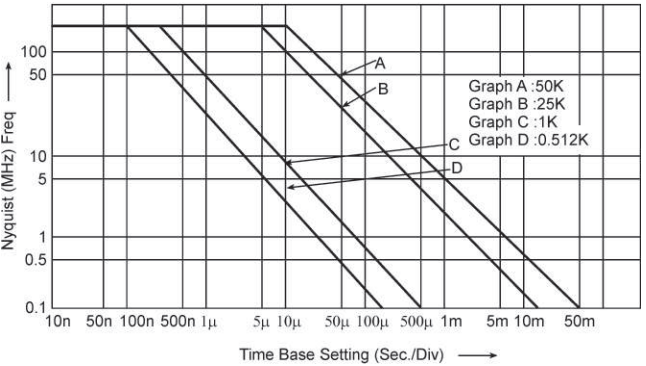
Hence, it must be accorded due importance when choosing one to meet your requirements. For a given time resolution, a longer memory enables events of longer duration to be recorded.
For instance, a DSO with a 1K memory can recorda1s transient with a time resolution of 1 ms, whereas a DSO with a 10K memory can record a 10 s long event with the same time resolution. In other words, for the same transient duration, longer memories give enhanced time resolution. Long memories also help in acquiring hard-to-catch signals and also minimize signal reconstruction distortion.
Vertical Accuracy and Resolution: The accuracy specification tells us how closely the measurement matches the actual value. The accuracy of a DSO is affected by various sources of error, including gain and offset errors, differential nonlinearity, quantization error and so on. The quantization error indirectly indicates vertical resolution, i.e. uncertainty associated with any reading or the ability of the oscilloscope to see small changes in amplitude measurements. Choosing a scope with fewer than eight bits of resolution is not recommended.
Resolution specification must not be considered in isolation from accuracy specification. For instance, more than eight bits of resolution is meaningless when the overall accuracy itself is ±1%. An eight-bit resolution gives a ±04% uncertainty, which is fairly acceptable if the overall accuracy is ±1%, as can be seen from following Table .
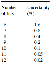
as a function of the number of bits.
Also, digital oscilloscopes with more than seven bits of resolution can resolve signal details better than visual measurements made with analogue oscilloscopes.
Importance of Specifications and Front-Panel Controls
It is very important to have a clear understanding of the performance specifications of oscilloscopes. The specification sheet supplied by the manufacturer contains scores of specifications. Each one of them is important in its own right and should not be ignored.
Although some of them explain only the broad features of the equipment and do not play a significant role as far as measurements are concerned, these are important when it is required to choose one for a given application. In fact, the performance specifications of an oscilloscope and the operational features of its front-panel controls cannot be considered in isolation. One complements the other.
Not only does the correct interpretation of specifications help in the selection of the right equipment for an intended application, their appreciation is almost a prerequisite to a proper understanding of the functional potential of front-panel controls.
Selection Criteria for Oscilloscopes
To sum up our discussion on the available oscilloscope types and the selection criteria for choosing the right one, it can be said that both analogue and digital oscilloscopes have their advantages and shortcomings. The suitability of a particular type must always be viewed in terms of intended application.
Although digital oscilloscopes can perform many functions that analogue versions cannot, analogue oscilloscope technology, too, has reached high performance standards. It is important to understand the critical specifications of each type and then decide whether it fits an intended application.
The key specifications to look for in analogue scopes are bandwidth, vertical sensitivity and accuracy, whereas the strength of a digital oscilloscope must be ascertained from its bandwidth, sample rate, vertical resolution, accuracy and memory length.
Oscilloscope Probes
The oscilloscope probe acts as a kind of interface between the circuit under test and the oscilloscope input. The signal to be viewed on the oscilloscope screen is fed to the vertical input (designated as the Y input) of the oscilloscope. An appropriate probe ensures that the circuit under test is not loaded by the input impedance of the oscilloscope vertical amplifier. This input impedance is usually 1 M Ω, in parallel with a capacitance of 10 – 50 pF.
The most commonly used general-purpose probes are the 1X, 10X and 100X probes. These probes respectively provide attenuation by factors of 1 (i.e. no attenuation), 10 and 100. That is, if we are measuring a 10 V signal with a 10X probe, the signal actually being fed to the oscilloscope input will be 1 V. 10X and 100X probes are quite useful for measuring high-amplitude signals.
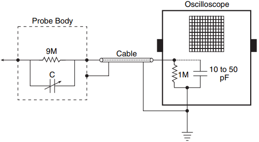
Another significant advantage of using these probes is that the capacitive loading on the circuit under test is drastically reduced. Refer to the internal circuit of the 10X probe as shown in Fig. 9. The RC time constant of the probe equals the input RC time constant of the oscilloscope.
Since the resistance of the probe is 9 times the input resistive component of the oscilloscope, in order to provide attenuation by a factor of 10, the probe capacitance has got to be smaller than the input capacitance of the scope by the same amount. As a result, the circuit under test with a 10X probe will never see a capacitance of more than 5 pF.
Oscilloscope Probe Compensation
The probe is compensated when its RC time constant equals the RC time constant of the oscilloscope input. With this, what we see on the screen of the scope is what we are trying to measure independent of the frequency of the input signal. If the probe is not properly compensated, the signal will be attenuated more than the attenuation factor of the probe at higher frequencies owing to reduction in the effective input impedance of the vertical input of the scope.
To check for probe compensation, the probe can be used to see the calibration signal (the CAL position on the front panel) available on the oscilloscope. If the probe is properly compensated, the CAL signal will appear in perfect rectangular shape [Fig. 20(a)] with no rounding-off of edges [Fig. 20(b)] or any spikes on fast transitions [Fig. 20(c)].
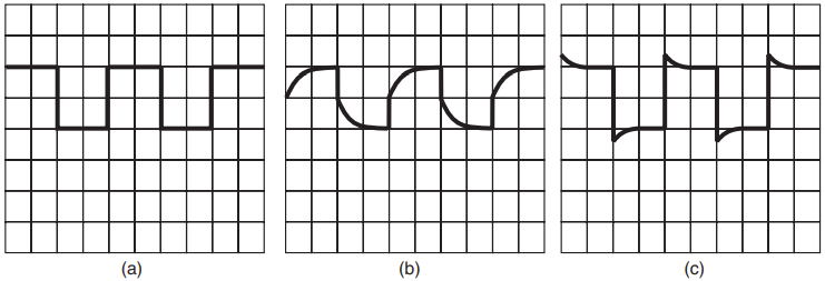
Rounding-off of edges indicates too little a probe capacitance, while spikes indicate too large a probe capacitance. The probe capacitance can be adjusted by turning a screw or rotating the probe barrel after loosening the locking nut (in some probes) to get a perfect calibration signal.
Related Posts
- Logic Gates
- Significance & Types of Logic Family
- Characteristics Parameters of Logic Families
- TTL Logic Family
- ECL Logic Family
- CMOS Logic Family
- Interfacing of Logic Families
- Microcontroller Architecture
- Components of Microcontroller
- Interfacing Devices with Microcontroller
- IC Based Multivibrator Circuits
- Astable, Monostable & Bistable Multivibrator
- Logic Analyser
- Types of Oscilloscope
- Frequency Synthesizers
- Frequency Counter